06-11 - Cornell University

WP 2006-11 May 2006

Working Paper Department of Applied Economics and Management Cornell University, Ithaca, New York 14853-7801 USA

Bubbles or Convenience Yields? A Theoretical Explanation with Evidence from Technology Company Equity Carve-Outs Vicki Bogan

It is the Policy of Cornell University actively to support equality of educational and employment opportunity. No person shall be denied admission to any educational program or activity or be denied employment on the basis of any legally prohibited discrimination involving, but not limited to, such factors as race, color, creed, religion, national or ethnic origin, sex, age or handicap. The University is committed to the maintenance of affirmative action programs which will assure the continuation of such equality of opportunity.

Bubbles or Convenience Yields? A Theoretical Explanation with Evidence from Technology Company Equity Carve-Outs Vicki Bogan∗ This Version: March 2006

Abstract This paper offers an alternative explanation for what is typically referred to as an asset pricing bubble. We develop a model that formalizes the Cochrane (2002) convenience yield theory of technology company stocks to explain why a rational agent would buy an “overpriced” security. Agents have a desire to trade but short-sale restrictions and other frictions limit their trading strategies and enable prices of two similar securities to be different. Thus, divergent prices for similar securities can be sustained in a rational expectations equilibrium. The paper also provides empirical support for the model using a sample of 1996 - 2000 equity carve-outs. (JEL: G10, G12, D50) Keywords: Asset Pricing, Rational Bubbles

∗

Department of Applied Economics and Management, 454 Warren Hall, Cornell University, Ithaca, NY 14853. Many thanks to Ignacio Palacios-Huerta, Herakles Polemarchakis, David Weil, and Sean Campbell for their insight, advice, and guidance. I would also like to thank Hazem Daouk, William Darity, Jr., Jay Ritter, and seminar participants at Brown University, Cornell University, and Fordham University for helpful comments and discussions. An additional thanks to Ignacio Palacios-Huerta for the data. All errors are my own. e-mail: [email protected], phone: 607-254-7219. c 2006. All rights reserved. Work in progress. °

1

1

Introduction

Historically, stock price bubbles have emerged in periods of productivity enhancing structural change. Market speculators gather around these theories regarding structural changes. If someone enters with a convincing story and line of thought for organizing otherwise confusing phenomena, he will attract speculative capital. For example, Internet company stocks were a gamble but since they were backed by the theory of an epochal change in technology that would alter the entire economic structure, investors found them attractive. Many economists, pundits, and commentators believe in the idea that irrational investors armed with this perspective and driven by a herd mentality forced the price of these stocks above their fundamental value. .......unsubstantiated belief systems, insubstantial wisps, do create bouts of irrational exuberance for significant periods of time, and these bouts ultimately drive the world economy.1 Yet, before we relegate the rapid rise and fall in Internet IPO stocks and other stocks to the bubble category driven by crowd psychology or investor ignorance, it makes sense to exhaust all economic explanations. In this paper we are interested in a rational alternative explanation for bubbles that has not yet been analytically formalized or empirically studied. Cochrane (2002) develops a convenience yield theory for the rise and fall of technology stocks and illustrates his point using a specific case example. This paper proposes a general theoretical model to formalize his theory and then provides empirical estimates to support the idea that the rise and fall of Internet/technology IPO stock prices may be explained by market frictions rather than investor irrationality. Initially, those in search of a rational alternative explanation for the high priced Internet IPO stocks during the Tech stock bubble attributed the high returns to the fact that IPOs historically have been shown to experience significant underpricing. This underpricing phenomenon has been well studied and documented in the economics literature (e.g., Michaely and Shaw (1994), Ghosh, 1

Shiller (2005), p. xiii.

2

Nag, and Sirmans (2000)). Numerous models have been offered to explain the situation (e.g., Rock (1986), Grinblatt and Hwang (1989), Allen and Faulhaber (1989)). However, Ritter and Welch (2002) argue that typical underpricing theories based on asymmetric information are unlikely to explain average first day returns of Internet stocks. Ljungqvist and Wilhelm (2003) suggest that, during the Internet bubble, changes in ownership structure (more fragmented ownership pre-IPO) and selling behavior (decrease in both frequency and magnitude of secondary sales by all categories of pre-IPO owners) generated a strong incentive to underprice. Yet, IPO underpricing cannot seem to account for the magnitude of the abnormal returns for Internet stocks. The abnormally high average returns for Internet/technology company IPOs far surpassed the typically high returns attributed to underpricing. Irrationality, heterogeneous agents, and short-sale constraints are other prominent explanations that have been applied to the Tech stock bubble. Under these assumptions, several theoretical models have been developed (e.g., Baker and Stein (2004), Scheinkman and Xiong (2003), Hong and Stein (2003), Abreu and Brunnermeier (2003)). There also has been significant empirical work (e.g., Jones and Lamont (2002), Ofek and Richardson (2003, 2002), Lamont and Thaler (2003)). None of these previously proposed bubble explanations sufficiently address all of the features of the Tech stock bubble (Cochrane, 2002). Cochrane (2002) clearly outlines the main bubble explanations in the literature and documents which of the characteristics of the Tech bubble they fail to capture. Not surprisingly, the convenience yield view proffered by Cochrane seems to be the most consistent with all of the characteristics of the technology/Internet IPO market. The convenience yield theory is an alternative explanation that does not rely on any form of agent/investor irrationality. Along the lines of Duffie, Gârleanu, and Pedersen (2002) which provides a framework for the price impact of the practice of shorting, the convenience yield theory of the technology stock market is connected to specific market search frictions. Cochrane (2002) posits that “few shares were available for trading, so the available shares gave a convenience yield: people were willing to hold them for a little while for short term trading, even though they knew that the shares were overvalued as a long term investment, just as people will briefly hold money 3

even though it depreciates.”2 Cochrane documents the analogy between technology stocks and conventional money demand using a specific IPO case example. Although Cochrane alludes to several possible theoretical models, he does not propose a specific model to justify his convenience yield theory. This paper tries to address this open issue in the literature by providing both a theoretical model and empirical estimates. This paper develops a three-period model based upon Boudoukh and Whitelaw (1993), which examines the issue of the value of liquidity in markets for riskless securities. The main purpose of our model is to explain how the prices for a group stocks (e.g., Internet company stocks) can be driven so significantly above the “fundamental value” that they would have had in a frictionless market. In this sense, the model attempts to reconcile an observed price bubble with the notion of efficient markets using the concept of convenience yields. The basic intuition of the threeperiod model is straight-forward: Agents are able to buy two similar types of securities. They are willing to pay more for one of the securities in period 1 even though they know that both security types will be worth the same amount in the last period. Rational agents do this because various market frictions limit their trading strategies and make one security type more valuable for trading purposes in period 2. Thus, this paper posits that there was a rational convenience yield for technology company stocks that was generated by a combination of economic factors (temporary supply shock, short-sale constraints, heterogeneous agents, and monopolistic market making). Given the tech stock demand3 , tech stocks futures were not a good substitute for actual tech stocks and these economic factors combined to make the spot price of some tech stocks high relative to the futures price. While we consider the model in the context of the Tech stock bubble, the model is general enough to be applied to any situation in which the identified market frictions are present. There is no question that the market for technology/Internet IPO stocks was characterized by many interesting features: (a) a large rise and then decline in prices, (b) prices not forecasting earnings, (c) short2

Cochrane (2002), p. 1. In terms of the economic rationale for the high tech stock demand, as Cochrane (2002) documents, there were no good substitutes for high frequency trading in this sector. 3

4

sales difficult and/or costly, (d) large dispersion of opinion about the stocks, (e) limited number of shares available, (f) high volume of trading, and (g) high volatility. If our model can explain the behavior of technology/Internet company bubble stocks, then it bodes well for explaining less severe overpricing/bubble situations. Empirical estimates to support the model are provided using a sample of equity carve-outs. For our group of stocks, we show that the convenience yields are generally larger and less volatile than those observed for commodities. However, our results also demonstrate that no unreasonably high convenience yield is needed to provide a plausible explanation for the Internet or other bubbles. The remainder of the paper proceeds as follows. Section 2 provides the rationale for why certain securities can be “overpriced” and why people are willing to buy these securities. Section 3 presents a three-period asset pricing model used to explain the convenience yield theory. Section 4 provides empirical estimates of convenience yields for a sample of technology companies and analyzes the relationship between market frictions and the convenience yields. Section 5 provides concluding remarks.

2

Why Investors Are Willing to Buy “Overpriced” Securities

The central prediction of the model is that agents are willing to buy securities that they know are “overpriced” for the purpose and convenience of short term trading. In our model, trade is motivated through shocks to endowments. Agents know that they are subject to this shock with some probability. Convenience is valued in this model because once agents realize their type, they will want to trade. Thus, they are willing to buy an “overpriced” security that will be more liquid for the purposes of short term trading. (i.e., It has a convenience yield.) Convenience yields for commodities are commonly observed. The convenience yield is the value associated with owning the actual item. In continuous time, F0 eyt = (S0 + U )ert where y is the convenience yield, F0 is the futures price, S0 is the spot price, U is the storage cost, r is the

5

discount rate, and t is time. The convenience yield reflects the market’s expectations concerning the future availability of the commodity/stock. The greater the possibility that shortages will occur, the higher the convenience yield. Thus, the convenience yield is a measure of the benefits from ownership of an asset that are not obtained by the holder of a long futures contract on the asset. Much of the literature related to convenience yields calculates the convenience yields for various commodities which are traded on futures markets (e.g., Considine (1997, 1992), Pindyck (1993)). Since by definition a convenience yield describes the residual price movement, the convenience yields for commodities typically move together with their prices (As shown by Pindyck (1993)). Sharp rises and declines in the convenience yields are observed. For commodities like lumber and heating oil, convenience yields can rise to well over 10% per month. Negative convenience yields also are observed.4 Only recently has the convenience yield concept been applied to more common institutional investments such as equities, cash, and bonds (See Smith (2000)).

3

Theoretical Framework

This section contains the basic model, based upon trade among heterogeneous agents. The key features of this model are: (i)limited supply of one asset, (ii) short sale constraints for this asset, (iii) heterogeneous agents, and (iv) market maker that sets bid and ask prices.5

3.1

Model Set-Up

Consider a three-period, (t = 1, 2, 3), endowment economy in which: • There are two types of stocks that can be traded: restricted stocks (sr ) and unrestricted stocks (su ). Restricted stocks are in small supply and thus have short sale constraints. Unrestricted 4

Pindyck (1993), p. 520-521. While these may not be appropriate assumptions for the secondary U.S. equities market, these are reasonable assumptions for the U.S. IPO market (See Section 3.6). 5

6

stocks have no short sale constraints. The prices are denoted pkit , where k = r (restricted stock) or k = u (unrestricted stock), i = a (ask price) or i = b (bid price). All prices are denominated in units of the consumption good. Although the stocks have different designations, we do not exclude cases in which they trade at identical prices. • All trade goes through a market maker at the market maker’s posted prices. The market maker holds no inventory and he must accept all orders at his posted prices. He must set prices to equate supply and demand in the markets for both securities. Additionally, the market maker sets bid-ask spreads based upon the different levels of institutional ownership observed.6 The market maker is interested only in period 2 revenues and does not engage in consumption. • Based on trading and consumption preferences, agents can be classified into four types: institutional traders, institutional investors, non-institutional traders, and non-institutional investors. Each period, agents receive an endowment, Yt . In the initial period, the agents know their primary type (institutional or non-institutional) but they do not know their secondary type (trader or investor). Agents receive endowments and take initial positions in the stock market based on their primary type, skjt , where j = I (institutional investor) or j = N (non-institutional investor). Institutional agents have a lower subsistence level of consumption7 , c¯j . c¯N = δ c¯I , where δ > 1. Without loss of generality we assume, srI1 = γsuI1 , where γ > 0. Agents maximize expected, time-separable, discounted von Neumann-Morgenstern utility. Agents can not make markets or hedge by forming coalitions. • In period 1, agents consume their endowments and/or invest in stocks. The issuer sells the total supply of stocks at ask prices that will clear the market. • At the beginning of the second period, agents realize their secondary type (endowment shock). Some agents want to buy stocks in the second period (investors/buyers) and others want to 6

Generally, bid-ask spreads are an increasing function of the levels of institutional ownership (Fehle, 2004). When the market makers sees a higher level of institutional ownership for a particular security, he will set a larger bid-ask spread (See Glosten and Milgrom (1985)). 7 Intuitively, we can think of institutional investors as not having to devote as great a proportion of their wealth/income to consumption of items like food, health care, etc.

7

sell stocks in the second period (traders/sellers). Investors pay ask prices and traders receive bid prices. The probability, qj , of being an investor is known. (Note that qI = qN .) • In period 2, agents adjust their portfolios subject to the short-sale constraint and consume their endowments plus net investment. • In period 3, agents consume their endowments plus the proceeds from the liquidation of their stocks.

3.2

Agents Optimization Problem

In equilibrium, the first order conditions from the agents’ utility maximization provide restrictions on the set of possible prices. The issuer and market maker then set prices given the agents’ optimal mapping from prices to stock holdings, in order to minimize cost within certain constraints. The agents maximize the expected value of the sum of discounted utility. Their problem in the first period is: maxct ,sk E1 t

i t−1 u(c + c¯ ) β t j t=1

hP 3

s.t. c1 ≤ Y1 − suj1 pua1 − srj1 pra1 − c¯j c2 ≤ Y2 − du (suj2 − suj1 )pua2 − dr (srj2 − srj1 )pra2 −(1 − du )(suj2 − suj1 )pub2 − (1 − dr )(srj2 − srj1 )prb2 − c¯j c3 ≤ Y3 + suj3 pu3 + srj3 pr3 − c¯j suj1 ≥ 0,

srj1 ≥ 0,

suj2 ≥ 0,

srj1 ≥ 0 (1)

where t = 1, 2, 3; k = r, u; j = I, N ; and ( 1 if suj2 ≥ suj1 , du = 0 otherwise.

( dr =

8

1 if srj2 ≥ srj1 , 0 otherwise.

Because of the complexity of first order conditions for problems containing indicator functions such as du and dr , it is necessary to analyze the problem within each class of equilibria and find parameter values for which solutions are supported. We assume the total supply of unrestricted stocks (Ω) is greater than the total supply of restricted stocks (κΩ). Thus, κ < 1. Also, the market clearing conditions must hold: u∗ su∗ I1 + sN 1 = Ω

(2)

r∗ sr∗ I1 + sN 1 = κΩ

(3)

r∗ u∗ r∗ u∗ r∗ qI su∗ BI2 + qI sBI2 + (1 − qI )sSI2 + (1 − qI )sSI2 + qN sBN 2 + qN sBN 2 r∗ +(1 − qN )su∗ SN 2 + (1 − qN )sSN 2 = (1 + κ)Ω

Tables 1 and 2 summarize the parameters used and the assumptions made.

9

(4)

10

Buyers/Investors Institutional Non-Institutional Sellers/Traders Institutional Non-Institutional

Y3 Y3 Y3 Y3

Y2S Y2S

Y1 Y1

Period 3

Y2B Y2B

Endowments Period 2

Y1 Y1

Period 1

Prices Period 2 bid ask prb2 pra2 pub2 pua2 Period 3 bid ask prb3 pub3 -

srI1 , suI1 srN 1 , suN 1

srI1 , suI1 srN 1 , suN 1

Period 1

srSI1 , suSI1 srSN 1 , suSN 1

srBI1 , suBI1 srBN 1 , suBN 1

0, 0 0, 0

0, 0 0, 0

Period 3

Total Supply κΩ Ω

Positions Period 2

Table 2: Summary of Agent Parameters

Restricted Stock Unrestricted Stock

Period 1 bid ask pra1 pua1

Table 1: Summary of Asset Parameters

c¯I c¯N

c¯I c¯N

Subsistence Level of Consumption

3.3

Equilibrium Concept

There is not one unique equilibrium solution for this model. Thus, it is important to define the concept of equilibrium for the purposes of this model. Definition 1: An equilibrium is a set of positive prices such that (i) markets clear in periods 1 and 2 (the supply of stocks equals the demand for stocks), and (ii) all agents maximize their discounted expected utility. In such a model, there can be an infinite number of equilibria that do not differ in any substantive manner. For example, if there exists an equilibrium in which no trade occurs in period 2 in the unrestricted stock with ask price pua2 = pˆ, then for all pua2 > pˆ we can achieve the same consumption, revenues, etc. We will consider all of these equilibria to be equivalent. Definition 2: Equivalent Equilibria are defined as those equilibria that support identical consumption streams and trading strategies for the agents and identical revenue streams for the issuer and the market maker, but differ in the equilibrium prices. To eliminate this multiplicity of equilibria, we will confine our attention in each case to the equilibrium, from the set of equivalent equilibria, with the lowest ask prices and highest bid prices. (i.e., the equilibrium with the smallest bid-ask spread.) Thus, we look at the equilibrium within the set of equivalent equilibrium with the highest convenience/liquidity and the smallest market maker profit.

3.4

Classification of Equilibria

The equilibria in the model can be divided into two categories: symmetric (equilibria with identical prices) and segmented (equilibria in which either bid prices or ask prices of the restricted and unrestricted stock differ at some point in time). Moreover, both the symmetric and the segmented equilibria can be further categorized based upon period 2 trade. 11

Symmetric Equilibria Equilibrium 1: No trade occurs. The bid price is set low enough and the ask price is set high enough such that none of the agents wish to trade. Equilibrium 2: Trade occurs but the constraint (for the sellers) on nonnegative holdings is not binding. For certain prices the sellers will wish to trade period 3 consumption for period 2 consumption by selling stocks and the buyers will wish to do the reverse. Equilibrium 3: Trade occurs and the constraint on nonnegative holdings is binding. As the bid price rises, the sellers wish to sell more of their holdings until the constraint on short-sales begins to bind. Segmented Equilibria Equilibrium 4: All restricted stocks held by sellers are traded but no unrestricted stocks are traded. The bid price on restricted stocks is set so that the constraint on nonnegative holdings binds and the bid price on the unrestricted stocks is low enough so that the sellers do not wish to sell any of their holdings of these stocks. Equilibrium 5: All of the restricted stocks held by the sellers are traded and some unrestricted stocks are traded. The nonnegative holdings constraint on the restricted stocks for the sellers binds and the bid and ask prices on the unrestricted stocks are set so that trade occurs. Equilibrium 6: All of the restricted and unrestricted stocks held by the sellers are traded. The period 2 bid prices on both types of stocks are high enough to induce the sellers to liquidate their holdings but these prices are not identical. It is important to note that a segmented equilibria in which only some of the restricted stocks held by the sellers are traded cannot be supported. Agents will not pay, in period 1, for convenience that they will never use. There is no distinction between a restricted stock and an unrestricted stock 12

Table 3: Equilibria Classifications and Trading Strategies Equilibrium

Type

Period 2 Trade in Restricted Stock

Period 2 Trade in Unrestricted Stock

1 2 3 4 5 6

Symmetric Symmetric Symmetric Segmented Segmented Segmented

None Some All All All All

None Some All None Some All

if both are certain to be held until the final period. Thus, in a rational expectations equilibrium, both assets must have identical prices if they are held until the final period. Table 3 summarizes the various types of equilibria.

3.5

Segmented Equilibria Example

The use of this model is motivated by the fact that its main assumptions match fairly closely to the institutional features and characteristics (volumes, etc.) of the Internet/technology company IPO market. Given this, we are interested in closely analyzing the segmented equilibria where the short-sale constraints are binding (Equilibria 4, 5, and 6). In each of these equilibria, we know that both the period 1 ask prices and the period 2 bid prices will differ across stocks (pua1 6= pra1 and pub2 6= prb2 ). Prices in the third period are normalized to one. The optimization problem is solved recursively. We consider a constant relative risk aversion (CRRA) form for the utility function, u(c) =

c1−α 1−α ,

where α represents the level of risk aversion. In

particular, we assume α = 1 (log utility) and the same discount rate for all agents (βsellers = βbuyers ) in order to obtain a more streamlined, closed form solution. A key component to the model set-up is that one group of agents wishes to sell stocks in the second period while the other group of agents buys stocks.8 Boudoukh and Whitelaw (1993) simply 8

For expected bubbles, endowments must be ex ante inefficient and every agent must be short-sale constrained. (Allen, Morris, & Postlewaite, 1993, p. 214).

13

assume that the marginal rate of substitution between periods 2 and 3 is higher for the sellers than for the buyers. This ensures in their model that the sellers always have more incentive than the buyers to sell stocks in period 2. Here trade is motivated by shocks to endowments where each group is distinguished by its endowments of the consumption good in each of the last two periods and the only way of transferring wealth across time is through stocks. However, Appendix B shows how the equilibrium results still hold if trade is motivated in a different way (e.g., different levels of risk aversion or different discount rates)9 .

3.5.1

Equilibrium 5: All Restricted Stocks and Some Unrestricted Stocks Are Traded

Equilibrium 5 is the most interesting equilibrium where trade takes place in both stocks. Thus, we will use this equilibrium to demonstrate the segmented solution to the optimization problem. The solution for this equilibrium is detailed in Appendix A. The first order conditions reduce to a system of three equations in five unknown prices, pua1 , pra1 , pa2 , pub2 , and prb2 . Recall that since buyers will not pay a premium in period 2 for restricted stock that they will hold until the final period, the ask prices for restricted and unrestricted stocks must be equal in the second period, pua2 = pra2 ≡ pa2 . We can specify two of the five prices and the other three prices will be determined in equilibrium. For this equilibrium, we set pub2 and prb2 , the bid prices in period 2. The ask price in period 2 can be written as pa2 =

pub2 (2qY3B

βq(Y2B − c¯I (1 + δ))pub2 + 2(1 − q)Y3S c¯I (1 + δ) + (1 + κ)Ω + (1 − q)βκΩ) − β(1 − q)(2Y2S + κΩprb2 c¯I (1 + δ)) (5)

9

For trade motivated by different discount rates, there is no endowment in the third period, all agents receive the same endowment in period 2, and one group of agents has a higher discount rate than the other group (βsellers < βbuyers ). Thus, one group wishes to consume more in the second period in order to maximize utility. For trade motivated by different levels of risk aversion, one group has a different level of risk aversion than the other group. The group with the higher elasticity of intertemporal substitution (EIS) is more willing to change their temporal allocations between periods 2 and 3.

14

While the period 1 ask prices of restricted and unrestricted stock are pua1 = pra1 =

(Y1 − c¯I )G T + 1+γ (γH + G) Ã (Y1 − c¯I )H 1− 0 T A0 F + 1+γ γH AF +

(6)

A0 F

T 1+γ G T 1+γ (γH

! + G)

(7)

where T

= suI1 + srI1

A0 = Y2B − c¯I + (Y3B − c¯I + T )pa2 F

= Y2S − c¯I +

γT r T pb2 + (Y3S − c¯I + )pu 1+γ 1 + γ b2

G = βq(1 + β)pa2 F + β(1 − q)(1 + β)pub2 A0 H = βq(1 + β)pa2 F + β(1 − q)(1 + β)prb2 A0

The choice of period 2 bid prices must be made in order to keep us in the selected class of equilibrium. As before, prices are assumed to be positive. Also, there is a restriction that sellers sell some, but u∗ r∗ not all, of their unrestricted stock, (0 < su∗ SI2 + sSN 2 < Ω) and all of their restricted stock, (sSj2 = u∗ 0, ∀j). Thus, equation (4) simplifies to qI s∗BI2 + qN s∗BN 2 + (1 − qI )su∗ SI2 + (1 − qN )sSN 2 = (1 + κ)Ω.

These restrictions imply the following ranges when setting the bid prices β(2Y2S − c¯I (1 + δ) + κΩprb2 ) β(2Y2S − c¯I (1 + δ) + κΩprb2 ) u < p < b2 2Y3S − c¯I (1 + δ) + Ω 2Y3S − c¯I (1 + δ) − βΩ prb2 ≥

2Y3S

2βY2S − c¯I (1 + δ) . − c¯I (1 + δ) + (1 − βκ)Ω

(8) (9)

We see from this segmented equilibrium case that divergent prices for similar securities can be sustained in a rational expectations equilibrium. The price segmentation is possible because heterogeneous agents have a desire to trade but specific market frictions limit their trading strategies and enable the prices of the two similar assets to be different in Period 1. (See Table 4 for a summary of asset prices.) 15

Table 4: Summary of Equilibrium 5 Asset Prices Bid Ask

3.5.2

Period 1 r pa1 > pua1

Period 2 prb2 > pub2 pra2 = pua2

Period 3 = pub3 = 1 -

prb3

Comparative Statics and Endogenously Generated Bid-Ask Spread

Another critical feature of our model is that market frictions can drive the market maker to set the bid prices such that one security is more liquid. Due to issues involving asymmetric information, when a market maker observes a higher level of institutional ownership for a particular security, he will set a larger bid-ask spread.10 A limited supply of one of the securities, rationing of that security, and different consumption preferences for the agents combine to create a situation which the market maker finds indistinguishable from the Glosten and Milgrom (1985) asymmetric information case when setting the bid-ask spread. As in Johnson (2004), the liquidity in this model (bid-ask spread) is driven by the supply of the stocks. Additionally, the liquidity is driven by the relative amount of institutional ownership in each stock which is directly affected by the subsistence level of consumption. From equation 9, we know that: ∂prb2 0. I ³ ´ ∂pu ∂pu ∂prb2 b2 · Since, ∂¯cb2 = > 0. Therefore, as the subsistence level of consumption decreases, the bid r ∂p ∂¯ cI I b2

price for the unrestricted stock (pub2 ) decreases (which increases the bid-ask spread since we have pra2 = pua2 ). Intuitively, this is consistent with the logic that as the subsistence level of consumption decreases, due to the limited supply of restricted stock (κ < 1), institutional investors would only be able to increase their investments by buying the unrestricted stock. This increase in the amount invested in unrestricted stock by institutional investors causes the bid-ask spread for unrestricted stock to increase (à la Glosten and Milgrom (1985)).11 Consequently, we will be in this equilibrium when there exists certain relationships between total supply of the stocks, endowments, discount rate, and total subsistence consumption.12 A Simple Numerical Example: It might be helpful to think about a crude but illustrative example of how market frictions could force one stock to have a larger proportion of institutional ownership. Consider a two period economy with two types of stocks (X & Y ) and two agents (A & B). There are 20 shares of stock X available and 150 shares of stock Y available. Both stocks have a price per share of $1. Both agents each have an initial endowment of $200. Agents engage in consumption and invest the remainder of their endowment in stocks. During the first period, agent A must use $90 for consumption while agent B must use $140 for consumption. If stock X is rationed due to its limited supply, agents A and B would each get 10 shares. Thus, agent A would buy 100 shares of Y and agent B would buy 50 shares of Y . This is precisely the type of difference in the proportion of institutional ownership that drives the different bid-ask spreads for the stocks.

11

Glosten & Milgrom, 1985 develop a model where bid-ask spreads are an increasing function of the level of institutional ownership. Recall that the period 2 ask prices for the unrestricted and restricted stocks must be the same. Given a relative increase in the institutional ownership of unrestricted stock, the period 2 bid price of the unrestricted stock will go down relative to the period 2 bid price of the restricted stock since the bid-ask spreads vary with institutional ownership. 12 Appendix C demonstrates that the assumption of the market maker setting bid-ask spreads based upon the different levels of institutional ownership is not inconsistent with a market maker who is only interested in period 2 revenue and does not engage in consumption.

17

3.6

Modeling Frictions versus Irrationality

This model exclusively focuses on the role of market frictions, leaving aside any forms of irrationality. Hence, the key assumptions in this economy are related to how the market frictions are modeled under conditions of rationality. For the price segmentation to be sustainable, short-sale constraints and a non-competitive market making mechanism are critical. If agents could costlessly sell stocks short in period 2 at the bid price (without any restrictions), then in equilibrium pub2 = prb2 and pua1 = pra1 . There would be no segmented equilibria.13 If market making was competitive, the period 2 bid-ask spreads on both stocks would be driven down to the market maker’s marginal cost of transacting. Excluding an ad hoc assumption of differential trading costs in the two stocks, a segmented equilibrium would not be sustainable. We were motivated by the fact that frictions such as short-sale constraints and non-competitive market making frictions actually were present in the Internet/technology company IPO market. Short-sales require one to borrow the stock before selling it. Since the stock of a recently IPO’d company was often simply not available for borrowing, short-sales were difficult and very costly. The Internet IPO market also had many similarities to a market with a non-competitive market making mechanism. Only certain firms and individuals had access to Internet IPOs. In an IPO market in general, “hot issues” are often rationed by the investment banker distributing them, with demand exceeding supply by a factor of as much as 20 (Allen and Faulhaber (1989)). The Internet/technology IPO market in the 1990s was no exception to this rule. Additionally, IPOs have lock-up periods which prevent the selling of shares of the stock for a minimum of three months after the IPO. Another important friction of the model is that different bid-ask spreads for the two types of stocks are endogenously generated as an increasing function of the level of institutional ownership. We assume that the institutional agents have a lower subsistence level of consumption which generates a lower bid-ask spread for the restricted stocks. Due to the lower bid-ask spread in period 2, 13

Boudoukh and Whitelaw (1993)

18

agents prefer to trade in the restricted stocks. In the presence of short-sale constraints, agents are willing to pay a premium for the restricted stock in period 1. This demand for the restricted stock enables price discrimination between restricted and unrestricted stocks. Without the lower bid-ask spread for restricted stocks, sellers in period 2 would not necessarily prefer to sell the restricted stock and the segmented equilibrium would not be sustainable. While Fehle (2004) demonstrates empirically that bid-ask spreads decrease with the level of ‘captive’ institutional owners, he also shows that for informed institutional investors, bid-ask spreads are positively related to institutional ownership. Additionally, we will show in the analytical section of this paper that the technology company IPOs did in fact have lower proportions of institutional ownership and had correspondingly smaller bid-ask spreads.

4

Empirical Estimates

The purpose of the previous section was to establish a theoretical basis for the convenience yield. Specific market frictions (short sale constraints, rationing of a stock in limited supply, and bid-ask spreads set as an increasing function of the level of institutional ownership), combine to create a convenience yield for a security. In this section, we want to empirically study markets, that are characterized by all of these frictions, for evidence on the size, temporal pattern, and factors influencing the convenience yield. We use data from technology/Internet company equity carve-out situations because they provide the most extreme examples of apparent “overpricing” and were subject to the specified market frictions. (e.g., Since the carve-outs we study were for less than 20% of the subsidiary shares, they were subject to severe short sale constraints.) They also provide a unique opportunity to observe different prices for identical assets.

19

4.1

Data

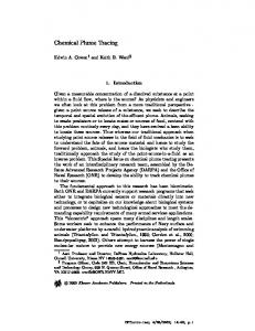
For our analysis we use the equity carve-out situations presented in Cochrane (2002) and Lamont and Thaler (2003). We use their April 1996 to August 2000 sample of every company in which there was an equity carve-out of less than 20 percent of subsidiary shares and the parent declared its intention to distribute the remaining shares. From that sample, we consider the subset of technology companies in which holders of a share of company A expected to receive x shares of company B by a certain date, yet the price of a share of company A stock was less than x times the price of a share of company B stock. Using Center for Research in Security Prices (CRSP) daily data, we first analyze prices, share turnover, bid-ask spreads, and distribution of returns for this set of companies in order to document some of the main characteristics of the market (large rise then decline in prices, high volume of trading, high volatility). For the purposes of calculating the convenience yields, we eliminate from the sample the one company in which the stock distribution was cancelled.14 This leaves us with a set of seven parent-subsidiary company pairs: Creative Computers/UBID, Daisytek International/PFSWeb, HNC Software/Retek, Methode Electronics/Stratos Lightwave, Odetics/ATL Products, 3Com/Palm, Tridex/TransAct Technologies. In all of these parent-subsidiary company pairs, it was cheaper to buy a share of the subsidiary stock “implicitly” by buying a share of the parent company than by buying a share of subsidiary stock directly (See Figure 2). The price of the subsidiary company would often exceed the price of the parent company for an extended period of time. This historical stock price data shows clear violations of the law of one price. The parent companies should be worth at least as much as their holdings in the subsidiary companies unless, as indicated previously, there is a convenience yield for the shares of the subsidiary company stock. From Figure 2, we observe the stock price pattern that is consistent with our theoretical model.15 We observe there was a large rise and then decline in the price of the newly IPO’d companies. We 14 15

With no distribution date, we lack a precise time frame (t) necessary for calculating the convenience yield. CRSP daily price data is based on bid/ask average.

20

Table 5: Average Proportion of Institutional Holdings from IPO Date to Distribution Date Avg. Quarterly Percentage of Institutional Ownership for: Unrestricted-Restricted Company Pairs

Unrestricted Stock (θu )

Restricted Stock (θr )

16.88% 6.80% 8.80% 6.40% 51.26% 15.11%

5.54% 3.62% 1.44% 1.69% 27.89% 10.75%

Creative Computers Inc. - UBID Inc. Daisytek International Corp. - PFSWeb Inc. HNC Software Inc. - Retek Inc. Methode Electronics Inc. - Stratos Lightwave Inc. 3Com Corp - Palm Inc. Tridex Corp. - TransAct Technologies Inc.

also see that the prices for the similar securities are different at the time of the initial IPOs (pu1 6= pr1 , as predicted by our model) but then return to comparable levels (pu3 = pr3 = 1). The 10-day moving average turnover for the subsidiary company stocks is usually above that for the parent company stock (See Figure 3). The standard deviations of returns for the subsidiary companies are higher than their corresponding parent company standard deviation of returns. Another key piece of empirical data supports one of the critical assumptions in our model. Using institutional holdings data from the Thomson Financial Securities Database (TFSD), we compute, on a quarterly basis,16 the total number of shares held by institutional investors as a percentage of the total shares outstanding (See Figure 4). We can see from Table 5, that the average level of institutional ownership for the subsidiary companies is always lower than for the parent companies.17 Also the bid-ask spreads for the subsidiary (restricted) stocks are usually lower than the bid-ask spreads for the parent (unrestricted) company stocks (See Figure 5). Finally, using LexisNexis information on the terms and dates of the stock distributions, we calculate the convenience yields implied by the differing prices in each parent-subsidiary company pair. Similar to the approach taken in the literature on commodity pricing (Pindyck, 1993), we use futures prices to calculate convenience yields. After the initial IPO for each subsidiary company, 16

Due to data limitations, we must use quarterly data. Average level calculated for period from the date of the IPO to the date that remaining shares of subsidiary stock were distributed to holders of the parent company stock (distribution date). 17

21

we treat the stock of the parent company as a future in the subsidiary company. The pricing data along with appropriate assumptions regarding discount rates and an assumption of zero storage costs can be used in the convenience yield equation, F0 eyt = S0 ert . Due to the length of time between the IPOs and the distribution dates, we calculate a daily rate for the convenience yields.18 A convenience yield for the stocks of these equity carve-outs is observed in the data. The implied convenience yields are shown in Figure 6. Relative to the convenience yields that we may see for commodities such as oil, copper, etc. (Gibson & Schwartz, 1989), the implied convenience yields for the subsidiary company stocks are larger and they follow a smoother path. The daily convenience yield is typically 0.5% - 1.0% (approximately 15% - 30% per month) until about a month before the distribution date and then the convenience yield declines sharply. Although larger than the convenience yields commonly observed for commodities, the magnitudes of the daily convenience yields are small. A 0.5% daily convenience yield can explain a greater than 100% difference in stock prices. We interpret these result as indicating, for short term trading, a small daily convenience yield can explain hugely divergent prices for similar assets. Additionally the observed convenience yield, that is clearly greater than zero, should be considered a particularly strong result given the assumption made regarding the future price for each subsidiary company. The fact that the value of the parent company is not extracted from the price of the subsidiary company future, means that we have understated the value of the convenience yields and explains why we can observe negative values for the convenience yields. In this sense, the convenience yields that we observe in the data may be considered to be the lower bounds. Our model shows that price differences can be supported by differences in the bid-ask spread. Additionally, our data does have evidence that these price differences could be accounted for by the associated savings in trading costs. For example, Figure 1 shows that the average daily convenience yields are lower than the average savings in round-trip transaction costs for the parent-subsidiary pairs. 18

For the discount rate, we use the daily one-year Treasury bill rate. However, a sensitivity analysis indicates that the shape and magnitude of the convenience yields are not sensitive to +/- 100% increases/decreases in r.

22

Figure 1: Difference Between Average Round Trip Transaction Cost Savings and Average Daily Convenience Yield (Holding Cost) 0.09

0.08

0.07

Percent

0.06

0.05

0.04

0.03

0.02

0.01

0.00 Creative Computers / UBID

Daisytek Int'l. / PFSWeb

HNC Software / Retek

Methode / Stratos

Odetics / ATL

3Com / Palm

Tridex / TransAct

Parent-Subsidiary Pairs

4.2

Relationship Between Market Frictions and Convenience Yield

Given that our theoretical model is predicated on several key market frictions, we analyze the relationship between these market frictions and the convenience yield. For each subsidiary (equity carve-out) company, we calculate a daily convenience yield starting from the day of its IPO ending with the day of the distribution of the remaining shares to its parent company shareholders. To understand the link between convenience yields and market frictions, we consider a simple regression model where the dependent variable is the convenience yield for each subsidiary company stock and the independent variables represent the various market frictions of the theoretical model. The independent variables include percent of institutional ownership, measure of relative daily liquidity, the number of shares outstanding, turnover19 , daily returns, parent company daily returns, and a measure of how “hot” the IPO issue was. We also include 1999 and 2000 year dummy variables to 19

A correlation analysis indicates no positive correlation (-0.0895) between the log of the number of shares outstanding and turnover.

23

Table 6: Coefficients from the Convenience Yield Regression Equation Intercept Institutional Ownership Relative Liquidity Log of Number of Shares Outstanding Turnover Daily Return: Carve-Out Daily Return: Parent Hot Issue Year 1999 Dummy Variable Year 2000 Dummy Variable

Coefficient

Standard Error

t-ratio

-0.1114 -0.0407 0.0011 0.0071 0.0162 0.0145 -0.0184 0.0000 -0.0028 -0.0184

0.0530 0.0139 0.0012 0.0034 0.0109 0.0162 0.0044 0.0002 0.0041 0.0064

-2.10 -2.92 0.90 2.09 1.48 0.90 -4.21 0.13 -0.68 -2.88

Number of Observations

950

R2 = 0.03

control for the fact that the independent company observations do overlap in time.20 A description of all of the variables used and how they are constructed can be found in Appendix D. The specification of this regression model is: CON V Y IELDit = β0 + β1 P ERCEN T IN ST OW Nij + β2 LIQU IDIT Yij + β3 SHARESOU Tij + β4 T U RN OV ERij + β5 RET U RNij + β6 P AREN T RET U RNij + β7 HOT ISSU Eij + β8 Y EAR1999ij + β9 Y EAR2000ij + ²ij , where ij is each company i’s observation for a particular day. Table 6 presents the parameter estimates.21 From these initial results, we see that percent of institutional ownership, shares outstanding, daily return of the parent company, and the year 2000 dummy variable are significant. The liquidity measure, turnover, daily return, the hot issue variable, and the year 1999 dummy were not significant.

20

We considered the use of an independent variable representing the market maker count, but could not use it due to data limitations. 21 Standard errors are adjusted to account for the fact that the observations are independent across companies but not within each company.

24

Table

7:

Coefficients from the Convenience (Data Adjusted for NonStationarities) Intercept Institutional Ownership Relative Liquidity Log of Number of Shares Outstanding Turnover Daily Return: Carve-Out Daily Return: Parent Hot Issue Year 1999 Dummy Variable Year 2000 Dummy Variable Number of Observations

Yield

Regression

Coefficient

Standard Error

t-ratio

0.0128 -0.0098 0.0002 -0.0008 0.0140 0.0009 -0.0057 0.0001 0.0035 -0.0041

0.0200 0.0040 0.0001 0.0013 0.0047 0.0017 0.0018 0.0001 0.0013 0.0013

0.64 -2.45 1.83 -0.66 2.95 0.53 -3.23 1.67 2.81 -3.17

828

Equation

R2 = 0.34

Robustness Check Our data set is not a true time series data set in that the daily information for each company covers a different period of time. However, we do observe “nonstationarities” in each of the convenience yields starting approximately one month prior to the scheduled distribution of the remaining subsidiary company shares by the parent company. To eliminate any spurious correlation based on these trends, we consider the same regression model but for each company we use the data starting from the day of its IPO ending with the day 30 calendar days prior to its distribution date. As we see in Table 7, removing the observed downward trends in the convenience yields strengthen the association between our independent variables and the convenience yield. We see that percent of institutional ownership, turnover, daily return of the parent company, and the year dummy variables are significant at the 5% level. The liquidity measure and the hot issue variable were significant at the 10% level. As expected, we observe that the percent of institutional ownership contributes negatively to the convenience yield, while being a hot issue and the liquidity measure contribute positively to the convenience yield.22 We also see that the year 22 This is consistent with our use of the hot issue variable as a proxy for the short sale constraints of our model. It is also consistent with our use of institutional ownership (driving lower bid prices) and differential bid-ask spreads in the theoretical model.

25

2000 dummy variable and the daily return of the parent company are negatively related to the convenience yield.23 The number of shares outstanding, and daily return were not significant. The results shown in Table 7 definitely support the idea that the frictions identified in our model do in fact contribute to the convenience yield of the stocks. These results are also quite compatible with our theoretical model’s use of these types of variables to generate the convenience yield. The percent of institutional ownership and turnover have the largest effect on the convenience yield. This is very encouraging given that, in our theoretical model, institutional ownership drives the difference in bid prices that generates the convenience yield. Additionally, we posit that investors pay a premium for the restricted stocks due to their desire for short term trading (turnover). The coefficients and mean values generated by our empirical model imply that a 1 percentage point decrease in the institutional ownership of a stock would increase the mean daily convenience yield by 0.0098 percent.

5

Conclusion

While most of the current literature focuses on irrationality as an explanation for asset pricing bubbles, this paper provides support for the existence of an alternative explanation. The theoretical basis provided for the convenience yield theory and the empirical estimates obtained of convenience yields for various Internet/technology companies support the idea that irrationality is not necessarily needed to explain the “Tech stock bubble”. From this perspective, the model and the data show how a combination of different market frictions, that were actually present in the Internet/technology IPO market, may cause the price of a technology company stock to rise above the value of a similar security and then return to its fundamental value. This temporary price segmentation is possible because agents have a desire to trade but short-sale restrictions limit their trading strategies and enable the prices of two similar securities to be different. While the 23

The negative relationship between convenience yield and parent company daily return makes intuitive sense in that as the parent company return increases, the parent company becomes more valuable relative to the subsidiary and hence the convenience yield would decrease.

26

empirical work of this paper focuses on the Tech stock bubble (1996 - 2000), a potential avenue for further research would be to perform similar analyses on a larger sample.24 There are some normative implications of our model and the corresponding empirical evidence. Historically, with regard to IPOs, there have been many restrictions and regulatory policies designed to keep prices from falling too low (e.g., Lock-up periods for IPOs are common.). However, there are no triggers to eliminate the restrictions if they push prices artificially high. Consequently, the conclusions derived from this area of research could be useful in shaping regulatory policy.

24

For the period between 1985 and 2000, Mitchell, Pulvino, and Stafford (2002) document 82 situations where the market value of a company is less than its subsidiary. This sample could be used for further tests of our model.

27

28

DAISYTEK INTERNATIONAL CORP

Time

PFSWEB INC

7/27/2002

1/27/2002

7/27/2001

1/27/2001

7/27/2000

CREATIVE COMPUTERS INC

1/27/2000

7/27/1999

1/27/1999

7/27/1998

1/27/1998

7/27/1997

1/27/1997

7/27/1996

1/27/1996

7/27/1995

1/27/1995

Stock Price

4/4/2000

1/4/2000

10/4/1999

7/4/1999

4/4/1999

1/4/1999

10/4/1998

7/4/1998

4/4/1998

1/4/1998

10/4/1997

7/4/1997

4/4/1997

1/4/1997

10/4/1996

7/4/1996

4/4/1996

1/4/1996

10/4/1995

7/4/1995

4/4/1995

Stock Price

Figure 2: Stock Prices

Creative Computers/.70488 and UBID

200

180

160

140

120

100

80

60

40

20

0

Time

UBID INC

Daisytek/0.81 and PFS Web

70

60

50

40

30

20

10

0

METHODE ELECTRONICS INC

29

Time

STRATOS LIGHTWAVE INC

9/3/2002

5/3/2002

1/3/2002

9/3/2001

5/3/2001

1/3/2001

9/3/2000

5/3/2000

1/3/2000

9/3/1999

H N C SOFTWARE INC

5/3/1999

1/3/1999

9/3/1998

5/3/1998

1/3/1998

9/3/1997

5/3/1997

1/3/1997

9/3/1996

5/3/1996

1/3/1996

9/3/1995

5/3/1995

1/3/1995

9/3/1994

5/3/1994

1/3/1994

Stock Price

6/21/2002

12/21/2001

6/21/2001

12/21/2000

6/21/2000

12/21/1999

6/21/1999

12/21/1998

6/21/1998

12/21/1997

6/21/1997

12/21/1996

6/21/1996

12/21/1995

6/21/1995

Stock Price


HNC Software/1.243 and Retek

120

100

80

60

40

20

0

Time

RETEK INC

Methode Electronics/1.5113 and Stratos Lightwave

60

50

40

30

20

10

0

3COM CORP

30

Time

PALM INC

10/3/2002

5/3/2002

12/3/2001

7/3/2001

2/3/2001

9/3/2000

4/3/2000

11/3/1999

6/3/1999

1/3/1999

ODETICS INC

8/3/1998

3/3/1998

10/3/1997

5/3/1997

12/3/1996

7/3/1996

2/3/1996

9/3/1995

4/3/1995

11/3/1994

6/3/1994

1/3/1994

Stock Price

9/3/1998

7/3/1998

5/3/1998

3/3/1998

1/3/1998

11/3/1997

9/3/1997

7/3/1997

5/3/1997

3/3/1997

1/3/1997

11/3/1996

9/3/1996

7/3/1996

5/3/1996

3/3/1996

1/3/1996

11/3/1995

9/3/1995

7/3/1995

5/3/1995

3/3/1995

1/3/1995

11/3/1994

9/3/1994

7/3/1994

5/3/1994

3/3/1994

1/3/1994

Stock Price


Odetics/1.1 and ATL Products

35

30

25

20

15

10

5

0

Time

A T L PRODUCTS INC

3Com/1.5 and Palm

100

90

80

70

60

50

40

30

20

10

0

TRIDEX CORP

31

TRANSACT TECHNOLOGIES INC Time

4/3/2000

1/3/2000

10/3/1999

7/3/1999

4/3/1999

1/3/1999

10/3/1998

7/3/1998

4/3/1998

1/3/1998

10/3/1997

7/3/1997

4/3/1997

1/3/1997

10/3/1996

7/3/1996

4/3/1996

1/3/1996

10/3/1995

7/3/1995

4/3/1995

1/3/1995

10/3/1994

7/3/1994

4/3/1994

1/3/1994

Stock Price


Tridex/1.005 and Transact Technologies

25

20

15

10

5

0

32

DAISYTEK INTERNATIONAL CORP.

Time

PFSWEB INC.

7/27/2002

1/27/2002

7/27/2001

1/27/2001

7/27/2000

CREATIVE COMPUTERS INC.

1/27/2000

7/27/1999

1/27/1999

7/27/1998

1/27/1998

7/27/1997

1/27/1997

7/27/1996

1/27/1996

7/27/1995

1/27/1995

Volume/Shares Issued (10-day moving avg.)

4/4/2000

1/4/2000

10/4/1999

7/4/1999

4/4/1999

1/4/1999

10/4/1998

7/4/1998

4/4/1998

1/4/1998

10/4/1997

7/4/1997

4/4/1997

1/4/1997

10/4/1996

7/4/1996

4/4/1996

1/4/1996

10/4/1995

7/4/1995

4/4/1995


Figure 3: Stock Turnover

Creative Computers and UBID

0.5

0.4

0.3

0.2

0.1

0

Time

UBID INC.

Daisytek International and PFS Web

0.20

0.18

0.16

0.14

0.12

0.10

0.08

0.06

0.04

0.02

0.00

METHODE ELECTRONICS INC.

33

Time

STRATOS LIGHTWAVE INC.

9/3/2002

5/3/2002

1/3/2002

9/3/2001

5/3/2001

1/3/2001

9/3/2000

5/3/2000

1/3/2000

9/3/1999

HNC SOFTWARE INC.

5/3/1999

1/3/1999

9/3/1998

5/3/1998

1/3/1998

9/3/1997

5/3/1997

1/3/1997

9/3/1996

5/3/1996

1/3/1996

9/3/1995

5/3/1995

1/3/1995

9/3/1994

5/3/1994

1/3/1994


6/21/2002

12/21/2001

6/21/2001

12/21/2000

6/21/2000

12/21/1999

6/21/1999

12/21/1998

6/21/1998

12/21/1997

6/21/1997

12/21/1996

6/21/1996

12/21/1995

6/21/1995



HNC Software and Retek

0.20

0.18

0.16

0.14

0.12

0.10

0.08

0.06

0.04

0.02

0.00

Time

RETEK INC.

Methode Electronics and Stratos Lightwave

0.20

0.18

0.16

0.14

0.12

0.10

0.08

0.06

0.04

0.02

0.00

3COM CORP.

34

Time

PALM INC.

9/3/2002

5/3/2002

1/3/2002

9/3/2001

5/3/2001

1/3/2001

9/3/2000

5/3/2000

1/3/2000

9/3/1999

5/3/1999

1/3/1999

ODETICS INC.

9/3/1998

5/3/1998

1/3/1998

9/3/1997

5/3/1997

1/3/1997

9/3/1996

5/3/1996

1/3/1996

9/3/1995

5/3/1995

1/3/1995

9/3/1994

5/3/1994

1/3/1994


9/3/1998

7/3/1998

5/3/1998

3/3/1998

1/3/1998

11/3/1997

9/3/1997

7/3/1997

5/3/1997

3/3/1997

1/3/1997

11/3/1996

9/3/1996

7/3/1996

5/3/1996

3/3/1996

1/3/1996

11/3/1995

9/3/1995

7/3/1995

5/3/1995

3/3/1995

1/3/1995

11/3/1994

9/3/1994

7/3/1994

5/3/1994

3/3/1994

1/3/1994



Odetics and ATL Products

0.20

0.18

0.16

0.14

0.12

0.10

0.08

0.06

0.04

0.02

0.00

Time

ATL PRODUCTS INC.

3Com Corp and Palm

0.20

0.18

0.16

0.14

0.12

0.10

0.08

0.06

0.04

0.02

0.00

TRIDEX CORP.

35 TRANSACT TECHNOLOGIES INC. Time

4/3/2000

1/3/2000

10/3/1999

7/3/1999

4/3/1999

1/3/1999

10/3/1998

7/3/1998

4/3/1998

1/3/1998

10/3/1997

7/3/1997

4/3/1997

1/3/1997

10/3/1996

7/3/1996

4/3/1996

1/3/1996

10/3/1995

7/3/1995

4/3/1995

1/3/1995

10/3/1994

7/3/1994

4/3/1994

1/3/1994



Tridex and Transact Technologies

0.20

0.18

0.16

0.14

0.12

0.10

0.08

0.06

0.04

0.02

0.00

Figure 4: Proportion of Institutional Ownership: Parent-Subsidiary Pairs Creative Computers and UBID

% Institutional Ownership

0.3 0.25 0.2 0.15 0.1 0.05

Dec-99

Distr. Date: 6-7-99

Sep-99

Jun-99

Mar-99

Dec-98

0

Time CREATIVE COMPUTERS INC

UBID INC



0.08 0.07 0.06 0.05 0.04 0.03 0.02 0.01

Dec-00

Distr. Date: 7-6-00

Sep-00

Jun-00

Mar-00

Dec-99

0

Time DAISYTEK INTERNATIONAL CORP

PFSWEB INC


0.1 0.08 0.06 0.04 0.02

Time HNC SOFTWARE INC

36

Distr. Date: 9-29-00 RETEK INC

Dec-00

Sep-00

Mar-00

Jun-00

0

Dec-99


0.12

Figure 4: Proportion of Institutional Ownership: Parent-Subsidiary Pairs Methode Electionics and Stratos Lightwave

0.07 0.06 0.05 0.04 0.03 0.02 0.01

Dec-01

Sep-01

Distr. Date: 4-28-01

Jun-01

Mar-01

Dec-00

Sep-00

Jun-00

0

Time METHODE ELECTRONICS INC

STRATOS LIGHTWAVE INC

3Com Corp and Palm


0.7 0.6 0.5 0.4 0.3 0.2 0.1

Dec-00


Sep-00

Mar-00

Jun-00

0

Time 3COM CORP

PALM INC

Tridex and Transact Technologies 0.3 0.25 0.2 0.15 0.1 0.05

TRIDEX CORP

Time TRANSACT TECHNOLOGIES INC

37

Dec-97

Sep-97


Jun-97

Mar-97

0

Dec-96



0.08

38

DAISYTEK INTERNATIONAL CORP.

Time

PFSWEB INC.

7/27/2002

1/27/2002

7/27/2001

1/27/2001

7/27/2000

CREATIVE COMPUTERS INC.

1/27/2000

7/27/1999

1/27/1999

7/27/1998

1/27/1998

7/27/1997

1/27/1997

7/27/1996

1/27/1996

7/27/1995

1/27/1995

Range ($) - 10 day moving avg.

4/4/2000

1/4/2000

10/4/1999

7/4/1999

4/4/1999

1/4/1999

10/4/1998

7/4/1998

4/4/1998

1/4/1998

10/4/1997

7/4/1997

4/4/1997

1/4/1997

10/4/1996

7/4/1996

4/4/1996

1/4/1996

10/4/1995

7/4/1995

4/4/1995


Figure 5: Bid Ask Spreads


1.2

1

0.8

0.6

0.4

0.2

0

Time

UBID INC.


1.4

1.2

1

0.8

0.6

0.4

0.2

0

METHODE ELECTRONICS INC.

39

Time

STRATOS LIGHTWAVE INC.

9/3/2002

5/3/2002

1/3/2002

9/3/2001

5/3/2001

1/3/2001

9/3/2000

5/3/2000

1/3/2000

9/3/1999

HNC SOFTWARE INC.

5/3/1999

1/3/1999

9/3/1998

5/3/1998

1/3/1998

9/3/1997

5/3/1997

1/3/1997

9/3/1996

5/3/1996

1/3/1996

9/3/1995

5/3/1995

1/3/1995

9/3/1994

5/3/1994

1/3/1994


6/21/2002

3/21/2002

12/21/2001

9/21/2001

6/21/2001

3/21/2001

12/21/2000

9/21/2000

6/21/2000

3/21/2000

12/21/1999

9/21/1999

6/21/1999

3/21/1999

12/21/1998

9/21/1998

6/21/1998

3/21/1998

12/21/1997

9/21/1997

6/21/1997

3/21/1997

12/21/1996

9/21/1996

6/21/1996

3/21/1996

12/21/1995

9/21/1995

6/21/1995



HNC Softward and Retek

2

1.8

1.6

1.4

1.2

1

0.8

0.6

0.4

0.2

0

Time

RETEK INC.


1.6

1.4

1.2

1

0.8

0.6

0.4

0.2

0

3COM CORP.

40

Time

PALM INC.

9/3/2002

5/3/2002

1/3/2002

9/3/2001

5/3/2001

1/3/2001

9/3/2000

5/3/2000

1/3/2000

9/3/1999

5/3/1999

1/3/1999

ODETICS INC.

9/3/1998

5/3/1998

1/3/1998

9/3/1997

5/3/1997

1/3/1997

9/3/1996

5/3/1996

1/3/1996

9/3/1995

5/3/1995

1/3/1995

9/3/1994

5/3/1994

1/3/1994


9/3/1998

7/3/1998

5/3/1998

3/3/1998

1/3/1998

11/3/1997

9/3/1997

7/3/1997

5/3/1997

3/3/1997

1/3/1997

11/3/1996

9/3/1996

7/3/1996

5/3/1996

3/3/1996

1/3/1996

11/3/1995

9/3/1995

7/3/1995

5/3/1995

3/3/1995

1/3/1995

11/3/1994

9/3/1994

7/3/1994

5/3/1994

3/3/1994

1/3/1994




4

3.5

3

2.5

2

1.5

1

0.5

0

Time

ATL PRODUCTS INC.

3Com Corp. and Palm

0.4

0.35

0.3

0.25

0.2

0.15

0.1

0.05

0

8/9/1995

TRIDEX CORP.

41

TRANSACT TECHNOLOGIES INC. Time

4/9/2000

2/9/2000

12/9/1999

10/9/1999

8/9/1999

6/9/1999

4/9/1999

2/9/1999

12/9/1998

10/9/1998

8/9/1998

6/9/1998

4/9/1998

2/9/1998

12/9/1997

10/9/1997

8/9/1997

6/9/1997

4/9/1997

2/9/1997

12/9/1996

10/9/1996

8/9/1996

6/9/1996

4/9/1996

2/9/1996

12/9/1995

10/9/1995



Tridex and Transact Technologies

0.8

0.7

0.6

0.5

0.4

0.3

0.2

0.1

0

Time

42

6/1/2000

5/25/2000

5/18/2000

5/11/2000

5/4/2000

4/27/2000

4/20/2000

4/13/2000

4/6/2000

3/30/2000

3/23/2000

3/16/2000

3/9/2000

3/2/2000

2/24/2000

2/17/2000

2/10/2000

2/3/2000

1/27/2000

1/20/2000

1/13/2000

1/6/2000

12/30/1999

12/23/1999

12/16/1999

12/9/1999

12/2/1999

Rate

6/3/1999

5/20/1999

5/6/1999

4/22/1999

4/8/1999

3/25/1999

3/11/1999

2/25/1999

2/11/1999

1/28/1999

1/14/1999

12/31/1998

12/17/1998

12/3/1998

Rate

Figure 6: Convenience Yields


0.02

0.01

0

-0.01

-0.02

-0.03

-0.04

-0.05

-0.06

-0.07

-0.08

Time


0.005

0

-0.005

-0.01

-0.015

-0.02

-0.025

Time

43

4/17/2001

4/3/2001

3/20/2001

3/6/2001

2/20/2001

2/6/2001

1/23/2001

1/9/2001

12/26/2000

12/12/2000

11/28/2000

11/14/2000

10/31/2000

10/17/2000

10/3/2000

9/19/2000

9/5/2000

8/22/2000

8/8/2000

7/25/2000

7/11/2000

6/27/2000

Rate

9/7/2000

8/24/2000

8/10/2000

7/27/2000

7/13/2000

6/29/2000

6/15/2000

6/1/2000

5/18/2000

5/4/2000

4/20/2000

4/6/2000

3/23/2000

3/9/2000

2/24/2000

2/10/2000

1/27/2000

1/13/2000

12/30/1999

12/16/1999

12/2/1999

11/18/1999

Rate



0.002

0

-0.002

-0.004

-0.006

-0.008

-0.01

-0.012

-0.014

-0.016

-0.018

Time


0.005

0

-0.005

-0.01

-0.015

-0.02

-0.025

-0.03

Time

44

7/13/2000

7/6/2000

6/29/2000

6/22/2000

6/15/2000

6/8/2000

6/1/2000

5/25/2000

5/18/2000

5/11/2000

5/4/2000

4/27/2000

4/20/2000

4/13/2000

4/6/2000

3/30/2000

3/23/2000

3/16/2000

3/9/2000

3/2/2000

Rate

3/7/1997

10/17/1997

10/10/1997

10/3/1997

9/26/1997

9/19/1997

9/12/1997

9/5/1997

8/29/1997

8/22/1997

8/15/1997

8/8/1997

8/1/1997

7/25/1997

7/18/1997

7/11/1997

7/4/1997

6/27/1997

6/20/1997

6/13/1997

6/6/1997

5/30/1997

5/23/1997

5/16/1997

5/9/1997

5/2/1997

4/25/1997

4/18/1997

4/11/1997

4/4/1997

3/28/1997

3/21/1997

3/14/1997

Rate



0.005

0

-0.005

-0.01

-0.015

-0.02

-0.025

-0.03

-0.035

Time

3Com and Palm

0.01

0.005

0

-0.005

-0.01

-0.015

-0.02

-0.025


Tridex and TransAct Technologies 0.005

0

Rate

-0.005

-0.01

-0.015

Time

45

2/23/1997

1/23/1997

12/23/1996

11/23/1996

10/23/1996

9/23/1996

8/23/1996

-0.02

Appendix A

Solving For Equilibrium 5

In this class of equilibria, the agents carry holdings suj1 and srj1 into period 2 and the period 2 problem for sellers is: maxsk u(c2 + c¯j ) + βu(c3 + c¯j ) t

s.t. c2 ≤ Y2S + (suSj2 − suSj1 )pub2 + srSj1 prb2 − c¯j c3 ≤ Y3S + suSj2 − c¯j ∀j

Recall that the agents realize their type prior to trade in period 2 and that the sellers sell all of their restricted stock and some of their unrestricted stocks in period 2 in this equilibrium. Under the same assumptions, the period 2 problem for the buyers is: maxsk u(c2 + c¯j ) + βu(c3 + c¯j ) t

s.t. c2 ≤ Y2B − (suBj2 − suBj1 )pua2 − (srBj2 − srBj1 )pra2 − c¯j c3 ≤ Y3B + suBj2 + srBj2 − c¯j ∀j

In analyzing this problem, we will use the fact that in equilibrium the period 2 ask prices of stocks are equal (pua2 = pra2 ≡ pa2 ) since the buyers of stocks in period 2 should make no distinction between the two types of stocks. This equality also means that the portfolio holdings of the buyers (suBj2 and srBj2 ) are not separately identified. Therefore, we maximize over their sum, sBj2 ≡ suBj2 + srBj2 to get the optimal total holdings of the buyers, s∗Bj2 . The above equations yield the following solutions for the optimal period 2 holdings:

=

β(Y2S − c¯j + srj1 prb2 ) (Y3S − c¯j − βsuj1 ) − (1 + β)pub2 (1 + β)

∀j

(A.1)

s∗Bj2 =

β(Y2B − c¯j ) (Y3B − c¯j − β(suj1 + srj1 )) − (1 + β)pa2 (1 + β)

∀j

(A.2)

su∗ Sj2

These equations are then used in the initial period problem, equation (1). The first order conditions for the initial period problem generate the following equations: 46

pua1 Y1 − c¯j − suj1 pua1 − srj1 pra1

= + +

pra1 Y1 − c¯j − suj1 pua1 − srj1 pra1

= + +

1 βqj pa2 ( 1+β )

(A.3)

Y2B − c¯j − (s∗Bj2 − suj1 − srj1 )pa2 1 β(1 − qj )pub2 ( 1+β ) u u r r Y2S − c¯j − (su∗ Sj2 − sj1 )pb2 + sj1 pb2 β β 2 (1 − qj ) 1+β

Y3S − c¯j + su∗ Sj2

+

β β 2 qj 1+β

Y3B − c¯j + s∗Bj2

∀j

1 ) βqj pa2 ( 1+β

(A.4)

Y2B − c¯j − (s∗Bj2 − suj1 − srj1 )pa2 1 β(1 − qj )prb2 ( 1+β ) u u r r Y2S − c¯j − (su∗ Sj2 − sj1 )pb2 + sj1 pb2 β β 2 (1 − qj )prb2 1+β

pub2 (Y3S − c¯j + su∗ Sj2 )

+

β β 2 qj 1+β

Y3B − c¯j + s∗Bj2

∀j

In equilibrium, for supply to equal demand in each period, equations (2) - (4) must also hold. The equations (2) - (4) and (A.1) - (A.4), define the equilibrium which has thirteen variables: suI1 , suN 1 , srI1 , srN 1 , sBI2 , sBN 2 , suSI2 , suSN 2 , pua1 , pra1 , pa2 , pub2 , and prb2 . Using appropriate substitutions, we can reduce the system to 3 equations in five unknowns. After substituting (2), (3), (A.1), and (A.2) into equations (A.3) and (A.4), simplifying and combining like terms we get the following equations:

pua1 Y1 − c¯I − suI1 pua1 − srI1 pra1

= +

pra1 Y1 − c¯I − suI1 pua1 − srI1 pra1

= +

Y2B Y2S Y2B Y2S

βqpa2 (1 + β) − c¯I + (Y3B − c¯I + suI1 + srI1 )pa2 β(1 − q)pub2 (1 + β) − c¯I + (Y3S − c¯I + suI1 )pub2 + srI1 prb2 βqpa2 (1 + β) − c¯I + (Y3B − c¯I + suI1 + srI1 )pa2 β(1 − q)prb2 (1 + β) − c¯I + (Y3S − c¯I + suI1 )pub2 + srI1 prb2

(A.5)

(A.6)

Substituting (A.1) and (A.2) into (4), simplifying and then substituting in (2) and (3) generates

47

2βq(Y2B − c¯I (1 + δ)) β(1 − q)(2Y2S + κΩprb2 − c¯I (1 + δ)) + + c¯I (1 + δ) = pa2 pub2

(A.7)

2qY3B + 2(1 − q)Y3S + (1 + κ)Ω + (1 − q)βκΩ

Thus, the system of equations (A.5) - (A.7) simplifies to equations (5) - (7).

B

Alternative Assumptions

We also will use equilibrium 5 to outline the solution under each set of assumptions. Recall that the agents realize their type prior to trade in period 2 and that the sellers sell all of their restricted stock and some of their unrestricted stocks in period 2 in this equilibrium.

B.1

Differing Discount Rates

In this scenario, there is no endowment in the third period and one group of agents (sellers) has a higher discount rate than the other group of agents (buyers) (βS < βB ). In solving the model, we assume log utility for both types of agents. In analyzing this problem, we use the fact that in equilibrium the period 2 ask prices of stocks are equal (pua2 = pra2 ≡ pa2 ), since the buyers of stocks in period 2 should make no distinction between the two types of stocks. This equality also means that the portfolio holdings of the buyers (suBj2 and srBj2 ) are not separately identified. Therefore, we maximize over their sum, sBj2 ≡ suBj2 + srBj2 ∀j to get the optimal total holdings of the buyers, s∗Bj2 . The first order conditions from the period 2 buyer and seller maximization problems yield the following solutions for the optimal period 2 holdings: su∗ Sj2 =

βS (Y2S − c¯j + srj1 prb2 ) Y3S − c¯j − βS suj1 − (1 + βS )pub2 (1 + βS )

∀j

(B.1a)

s∗Bj2 =

βB (Y2B − c¯j ) Y3B − c¯j − βB (suj1 + srj1 ) − (1 + βB )pa2 (1 + βB )

∀j

(B.1b)

48

These equations are then used in the initial period problem, equation (1). max

ln(Y1 − c¯I − suI1 pua1 − srI1 pra1 ) + ln(Y1 − c¯N − suN 1 pua1 − srN 1 pra1 ) +βB qI ln(Y2B − c¯I − s∗BI2 pa2 + (suI1 + srI1 )pa2 ) +βB qN ln(Y2B − c¯N − s∗BN 2 pa2 + (suN 1 + srN 1 )pa2 ) u u r r +βS (1 − qI )ln(Y2S − c¯I − (su∗ SI2 − sI1 )pb2 + sI1 pb2 ) u u r r +βS (1 − qN )ln(Y2S − c¯N − (su∗ SN 2 − sN 1 )pb2 + sN 1 pb2 ) 2 2 +βB qI ln(Y3B c¯I + s∗BI2 ) + βB qN ln(Y3B c¯N + s∗BN 2 ) 2 S u∗ +βS2 (1 − qI )ln(Y3S − c¯I + su∗ SI2 ) + βS (1 − qI )ln(Y3 − c¯I + sSI2 )

In equilibrium, for supply to equal demand in each period, equations (2) - (4) must also hold. The first order conditions along with the market clearing conditions generate the following equations (after appropriate substitutions and simplifications are made): pua1 Y1 − c¯j − suj1 pua1 + srj1 pra1

= +

pra1 Y1 − c¯j − suj1 pua1 + srj1 pra1

= +

βB qj pa2 (1 + βB ) Y2B − c¯j + (Y3B − c¯j + suj1 + srj1 )pa2 Y2S

βS (1 − qj )pub2 (1 + βS ) − c¯j + (Y3S − c¯j + suj1 )pub2 + srj1 prb2

Y2B

βB qj pa2 (1 + βB ) − c¯j + (Y3B − c¯j + suj1 + srj1 )pa2

Y2S

βS (1 − qj )prb2 (1 + βS ) − c¯j + (Y3S − c¯j + suj1 )pub2 + srj1 prb2

(B.1c) ∀j (B.1d) ∀j

βB (1 + βS )(qI (Y2B − c¯I ) + qN (Y2B − c¯N )) pa2 S r βS (1 + βB )((1 − qI )(Y2 − c¯I + sI1 prb2 ) + (1 − qN )(Y2S − c¯N + srN 1 prb2 )) + pub2 = (1 + βB )(1 + βS )(1 + κ)Ω +(1 + βS )[qI (Y3B − c¯I − βB (suI1 + srI1 )) + qN (Y3B − c¯N − βB (suN 1 + srN 1 ))] +(1 + βB )[(1 − qI )(Y3S + c¯I + βS suI1 ) + (1 − qN )(Y3S + c¯N + βS suN 1 )] (B.1e) As before, this system of equations defines the equilibrium.

B.2

Differing Levels of Risk Aversion

In this scenario, we assume the same discount rate for all agents but that one group of agents (sellers) is less risk averse than the other group of agents (buyers). To solve the model, we consider 49

1−α

a CRRA utility function (u(c) = c1−α ) where buyers have a higher level of risk aversion (α = 2) and sellers have log utility (α = 1). Given these assumptions regarding risk aversion, sellers have a higher elasticity of intertemporal substitution (EIS) and thus are more motivated to change their temporal allocations between periods 2 and 3. Again we use the fact that in equilibrium the period 2 ask prices of stocks are equal (pua2 = pra2 ≡ pa2 ), since the buyers of stocks in period 2 should make no distinction between the two types of stocks. This equality also means that the portfolio holdings of the buyers (suBj2 and srBj2 ) are not separately identified. Therefore, we maximize over their sum, sBj2 ≡ suBj2 + srBj2 ∀j to get the optimal total holdings of the buyers, s∗Bj2 . The first order conditions from the period 2 buyer and seller maximization problems yield the following solutions for the optimal period 2 holdings: su∗ Sj2

=

β(Y2S − c¯j + srj1 prb2 ) Y3S c¯j − βsuj1 − (1 + β)pub2 (1 + β) 1

s∗Bj2

=

∀j

(B.2a)

∀j

(B.2b)

1

Y2B + pa2 (suj1 + srj1 ) − Y3B ( pβa2 ) 2 − c¯j (1 − ( pβa2 ) 2 + pa2 ) 1

( pβa2 ) 2 + pa2

These equations are then used in the initial period problem, equation (1). max

− (Y1 − c¯I − suI1 pua1 − srI1 pra1 )−1 − (Y1 − c¯N − suN 1 pua1 − srN 1 pra1 )−1 + ln(Y1 − c¯I − suI1 pua1 − srI1 pra1 ) + ln(Y1 − c¯N − suN 1 pua1 − srN 1 pra1 ) − βqI (Y2B − c¯I − s∗BI2 pa2 + (suI1 + srI1 )pa2 )−1 − βqN (Y2B − c¯N − s∗BN 2 pa2 + (suN 1 + srN 1 )pa2 )−1 u u r r + β(1 − qI )ln(Y2S − c¯I − (su∗ SI2 − sI1 )pb2 + sI1 pb2 ) u u r r + β(1 − qN )ln(Y2S − c¯N − (su∗ SN 2 − sN 1 )pb2 + sN 1 pb2 )

− β 2 qI (Y3B − c¯I + s∗BI2 )−1 − β 2 qN (Y3B − c¯N + s∗BN 2 )−1 2 S u∗ + β 2 (1 − qI )ln(Y3S − c¯I + su∗ N + sSN 2 ) SI2 ) + β (1 − qN )ln(Y3 − c¯

In equilibrium, for supply to equal demand in each period, equations (2) - (4) must also hold. The first order conditions along with the market clearing conditions generate the following equations (after appropriate substitutions and simplifications are made): pua1 (1 + Y1 − c¯j − suj1 pua1 − srj1 pra1 ) (Y1 − c¯j − suj1 pua1 − srj1 pra1 )2

1

= +

pra1 (1 + Y1 − c¯j − suj1 pua1 − srj1 pra1 ) (Y1 − c¯j − suj1 pua1 − srj1 pra1 )2

(Y2B Y2S

βqj pa2 (1 + (βpa2 ) 2 )2 − c¯j + pa2 (Y2B − c¯j + suj1 + srj1 ))2

β(1 − qj )pub2 (1 + β) − c¯j + srj1 prb2 + pub2 (Y3S − c¯j + suj1 )

(B.2c) ∀j

1

= +

(Y2B Y2S 50

βqj pa2 (1 + (βpa2 ) 2 )2 − c¯j + pa2 (Y3B − c¯j + suj1 + srj1 ))2

β(1 − qj )prb2 (1 + β) − c¯j + srj1 prb2 + pub2 (Y3S − c¯j + suj1 )

(B.2d) ∀j

1

(1 + β)qI (Y2B − c¯I + pa2 (suI1 + srI1 ) − (Y3B − c¯I )( pβa2 ) 2 )

+

1

( pβa2 ) 2 + pa2 1

(1 + β)qN (Y2B − c¯N + pa2 (suN 1 + srN 1 ) − (Y3B − c¯N )( pβa2 ) 2 ) 1

( pβa2 ) 2 + pa2

+

β(1 − qI )(Y2S − c¯I + srI1 prb2 ) + β(1 − qN )(Y2S − c¯N + srN 1 prb2 ) = pub2 (1 − qI )(Y3S − c¯I − βsuI1 ) + (1 − qN )(Y3S − c¯N − βsuN 1 ) + (1 + β)(1 + κ)Ω (B.2e) As before, this system of equations defines the equilibrium.

51

C

Equilibrium 5 Market Maker Revenue - Numerical Analysis

As detailed in section 3.5.1, the market maker sets the two period 2 bid prices and the period 2 ask price is determined in equilibrium. Also, the market maker sets bid-ask spreads based upon the different levels of institutional ownership observed. Using a numerical analysis approach, we demonstrate that this assumption is not inconsistent with a market maker who is only interested in period 2 revenue and does not engage in consumption. The market maker’s revenue function is: max(pa2 − prb2 )vol(r) + (pa2 − pub2 )vol(u) where vol(r) is the per capital volume of restricted stock that is sold in period 2, and vol(u) is the per capita volume of unrestricted stock that is sold in period 2. It is prohibitively complicated to calculate the market maker revenue within this class of equilibrium in closed form and to optimize analytically. Instead, we utilize a numerical analysis approach to determine estimates for the parameters that maximize market maker revenue. Using these values for β, κ, Ω, q, δ, c¯, Y2B , Y2S , Y3B , and Y3S † , in Figure 7 we graph the revenue function over a range of values for prb2 and pub2 . This graphically illustrates that under certain conditions, the market maker can increase his revenue by lowering pub2 for any given prb2 (i.e., setting a larger bid-ask spread for the unrestricted stock when it has a larger level of institutional ownership). See also Figure 8.

†

β = 0.9, κ = 0.1, Ω = 0.2, q = 0.4, δ = 1.1, c¯ = 20, Y2B = 120, Y2S = 20, Y3B = 20, Y3S = 20

52

Figure 7: Feasible Equilibria

2

prb2

1.5

1

0.5

0 0.1 30 20

0.05

10 0 0

pub2

−10 −20

Revenue

Figure 8: Market Maker Revenue and Unrestricted Stock Period 2 Bid Price 0.1 0.09 0.08 0.07

pub2

0.06 0.05 0.04 0.03 0.02 0.01 0 −20

−15

−10

−5

0 5 Revenue

53

10

15

20

25

D

Description of Variables Used in Empirical Analysis • Percent Institutional Ownership - Total number of shares held by institutional investors as a percentage of total shares outstanding (computed quarterly). Due to data limitations, we must use average quarterly figures as a proxy for daily percent of institutional ownership. • Relative Liquidity - Daily average bid-ask spread for parent company minus the daily average bid-ask spread for subsidiary company (carve-out). • Log of Number of Shares Outstanding - The log of the total number of publicly held shares (carve-out). • Share Turnover - The total number of shares traded per day divided by the total number of shares outstanding (carve-out). • Daily Return of Carve-Out Company - The daily change in the total value of an investment in the stock per dollar of initial investment. • Daily Return of Parent Company - The daily change in the total value of an investment in the stock per dollar of initial investment. • Hot Issue - A variable indicating the total number of LexisNexis hits for the subsidiary company for the period one month prior to its IPO. (We use the log of this number of news articles about the upcoming IPO as an indication of how “hot” the IPO issue was.) • 1999 Year Dummy Variable - A dummy variable set to 1 if the year is 1999 and 0 otherwise. • 2000 Year Dummy Variable - A dummy variable set to 1 if the year is 2000 and 0 otherwise.

54

References Abreu, D., & Brunnermeier, M. K. (2003). “Bubbles and Crashes.” Econometrica, 71 (1), 173-204. Allen, F., & Faulhaber, G. R. (1989). “Signaling by Underpricing in the IPO Market.” Journal of Financial Economics, 23, 303-323. Allen, F., Morris, S., & Postlewaite, A. (1993). “Finite Bubbles with Short Sale Constraints and Asymmetric Information.” Journal of Economic Theory, 61, 206-229. Baker, M., & Stein, J. C. (2004). “Market Liquidity as a Sentiment Indicator.” Journal of Financial Markets, 7 (3), 271-299. Boudoukh, J., & Whitelaw, R. F. (1993). “Liquidity as a Choice Variable: A Lesson from the Japanese Government Bond Market.” Review of Financial Studies, 6 (2), 265-292. Cochrane, J. H. (2002). “Stocks as Money: Convenience Yield and the Tech-Stock Bubble.” (Manuscript, Graduate School of Business, University of Chicago) Considine, T. J. (1992). “A Short-Run Model of Petroleum Product Supply.” Energy Journal, 13 (2), 61-91. Considine, T. J. (1997). “Inventories Under Joint Production: An Empirical Analysis of Petroleum Refining.” Review of Economics and Statistics, 79 (3), 493-502. Duffie, D., Gârleanu, N., & Pedersen, L. H. (2002). “Securities Lending, Shorting, and Pricing.” Journal of Financial Economics, 66, 307-339. Fehle, F. (2004). “Bid-Ask Spreads and Institutional Ownership.” Review of Quantitative Finance and Accounting, 22 (4), 275-292. Ghosh, C., Nag, R., & Sirmans, C. (2000). “A Test of the Signaling Value of IPO Underpricing with REIT IPO-SEO Pairs.” Journal of Real Estate Finance and Economics, 20 (2), 137-154. Gibson, R., & Schwartz, E. S. (1989). “Stochastic Convenience Yield and the Pricing of Oil Contingent Claims.” Journal of Finance, 45 (3), 959-976. Glosten, L. R., & Milgrom, P. R. (1985). “Bid, Ask and Transaction Prices in a Specialist Market with Heterogeneously informed traders.” Journal of Financial Economics, 14, 71-100. Grinblatt, M., & Hwang, C. Y. (1989). “Signaling and the Pricing of New Issues.” Journal of Finance, 44 (2), 393-420. Hong, H., & Stein, J. C. (2003). “Differences of Opinion, Short-Sales Constraints, and Market Crashes.” Review of Financial Studies, 16 (2), 487-525. Johnson, T. C. (2004). “Dynamic Liquidity in Endowment Economies.” Business School)

55

(Manuscript, London

Jones, C. M., & Lamont, O. A. (2002). “Short Sale Constraints and Stock Returns.” Journal of Financial Economics, 66 (2-3), 207-239. Lamont, O. A., & Thaler, R. H. (2003). “Can the Market Add and Subtract? Mispricing in Tech Stock Carve-Outs.” Journal of Political Economy, 111 (2), 227-268. Ljungqvist, A., & Wilhelm, W. J. (2003). “IPO Pricing in the Dot-Com Bubble.” Journal of Finance, 58 (2), 723-752. Michaely, R., & Shaw, W. H. (1994). “The Pricing of Initial Public Offerings: Tests of AdverseSelection and Signaling Theories.” Review of Financial Studies, 7 (2), 279-319. Mitchell, M., Pulvino, T., & Stafford, E. (2002). “Limited Arbitrage in Equity Markets.” Journal of Finance, 57 (2), 551-584. Ofek, E., & Richardson, M. (2002). “The Valuation and Market Rationality of Internet Stock Prices.” Oxford Review of Economic Policy, 18 (3), 265-287. Ofek, E., & Richardson, M. (2003). “Dotcom Mania: The Rise and Fall of Internet Stock Prices.” Journal of Finance, 58 (3), 1113-1137. Pindyck, R. S. (1993). “The Present Value Model of Rational Commodity Pricing.” Economic Journal, 103 (418), 511-530. Ritter, J. R., & Welch, I. (2002). “A Review of IPO Activity, Pricing, and Allocations.” Journal of Finance, 57 (4), 1795- 1828. Rock, K. (1986). “Why New Issues are Underpriced.” Journal of Financial Economics, 15, 187-212. Scheinkman, J., & Xiong, W. (2003). “Overconfidence and Speculative Bubbles.” Journal of Political Economy, 111 (6), 1183- 1219. Shiller, R. J. (2005). Irrational Exuberance (2 ed.). Princeton, N.J.: Princeton University Press. Smith, A. (2000). “Introduction to Convenience Yields.” Investment Conference)

56

(Manuscript, Prepared for the 2000