arXiv:q-bio/0703020v1 [q-bio.PE] 8 Mar 2007
Chromosome-Length-Scaling in Haploid, Asexual Reproduction P.M.C. de Oliveira Instituto de F´ısica Universidade Federal Fluminense av. Litorˆ anea s/n, Boa Viagem, Niter´ oi, Brasil 24210-340 e-mail addresses:
[email protected] Abstract We study the genetic behaviour of a population formed by haploid individuals which reproduce asexually. The genetic information for each individual is stored along a bit-string (or chromosome) with L bits, where 0-bits represent the wild-type allele and 1-bits correspond to harmful mutations. Each newborn inherits this chromosome from its parent with some few random mutations: on average a fixed number m of bits are flipped. Selection is implemented according to the number N of 1-bits counted along the individual’s chromosome: the smaller N the higher the probability an individual has to survive a new time step. Such a population evolves, with births and deaths, and its genetic distribution becomes stabilised after many enough generations have passed. The question we pose concerns the procedure of increasing L . The aim is to get the same distribution of relative genetic loads N/L among the equilibrated population, in spite of a larger L . Should we keep the same mutation rate m/L for different values of L ? The answer is yes, which intuitively seems to be plausible. However, this conclusion is not trivial, according to our simulational results: the question involves also the population size.
1
1
Introduction
A natural way for evolution is to increase the chromosome length in order to make space for more genetic information. However, Nature seems to impose a maximum possible chromosome length, as inferred from at least two general observations. First, all big animals present the same order of magnitude for their chromosome lengths. Second, the genetic information for these animals is spread over more-than-one chromosome pairs (23 for humans), instead of a single, long one. This broken-information storage strategy demands an extra cost, a coordinated regulatory mechanism triggering the simultaneous copy of the various chromosomes at reproduction or cell division. Therefore, some unavoidable obstacle should exist, which prevents Nature to follow the simpler rule of increasing the length of a single chromosome. On the other hand, during reproduction, the chemical machinery which performs DNA duplication works as a zipper, scanning the one dimensional chromosome chain, basis after basis. Thus, the total number m of “errors” (i.e. mutations appearing in offspring as compared to parents) should be proportional to the chromosome length L , on average. Therefore, by increasing L , this linear behaviour indicates that one should keep the same mutation rate m/L : this procedure is then supposed to yield the same genetic quality for the whole population, in spite of the larger L . In order to test these ideas, we decided to simulate on computers a very simple model where each individual carries a single chromosome represented by a bit-string with L bits. Each bit can appear in either of two forms, 0 or 1 . The allele represented by a 0-bit is the wild type, whereas a 1-bit corresponds to some harmful mutation. In this work, we treat the case of haploid individuals, the genetic information stored along a single bit-string. In another related work [1] we treat diploid, sexual reproducing populations with crossings and recombination, and the results and conclusions are completely different (preliminary results can be found in [2]). The model is designed in order to keep only the fundamental ingredients of genetic inheritance and Darwinian evolution: random mutations performed at birth, and natural selection. All other biological issues which have no direct influence during the very moment of reproduction are ignored, as, for instance, the various correlations and inhomogeneities along the chromosome, the various phases during embryo development, the metabolism during life, etc. Instead, selection is implemented by taking into account just one phenotype: the number N of harmful alleles, i.e. 1-bits counted along the individual’s chromosome. It is a minimalist model, not a reductionist one, because we do not divide the problem into smaller, separate pieces neither in space nor in time (see [4]). This distinction between minimalism and reductionism is of fundamental importance in what concerns the size- and time-scaling behaviour which leads to the criticality observed in evolutionary systems [2]. We keep in the computer memory the chromosome (bit-string) of each individual belonging to a population (in reality, the number of 1-bits is enough). The total number P of individuals is kept fixed by controlling the number of 2
deaths equal to the number of births at each new time step: a fraction b of the population dies, while another fraction also equal to b of newborns are generated by random parents chosen among the survivors. At each time step, we perform two successive sub-steps, first deaths and then births. The death sub-step contains the selection ingredient [3]: an individual with N + 1 harmful alleles ( 1-bits) along its chromosome survives with a smaller probability than another individual with N harmful alleles. Let’s call x the ratio between these two probabilities, x = P (N + 1)/P (N ) , and let’s also consider x independent of N = 0, 1, 2 . . . L (this assumption is equivalent to adopt an exponential decay for the survival probability as a function of N ). The same x is also adopted as the survival probability for individuals with N = 0 . Of course, the value of x should be strictly smaller than 1, otherwise nobody dies and the population does not evolve. Let’s now describe the first sub-step corresponding to deaths. First, we count the number H(N ) of individuals with N harmful alleles. Then, we solve the polynomial equation L X
H(N ) xN +1 = (1 − b) P
(1)
N =0
getting the value of x . We adopted b = 0.02 , i.e. 2% of the population die each new time step. Other not-too-large values (1%, 3% , etc) can also be adopted with the same results, since the role of b is only to fix a convenient time scale, the time interval between two successive snapshots of a movie describing the evolving population. As b is a small fraction, x is always near 1 (in fact, 1 − b ≤ x < 1 ). Now, for each individual i , we toss a random number r in between 0 and 1 : if r < xNi +1 , then this individual survives, where Ni counts the number of harmful alleles along its chromosome; otherwise, this individual dies and is excluded from the population. After applying this death roulette to the whole population, the number of survivors is (1 − b) P , on average. The second sub-step corresponds to births in exactly the same number of deaths occurred during the first. For each newborn we toss a random parent among the survivors. Then, we copy its chromosome and perform mutations on the copy. Each mutation is a bit which is flipped (from 0 to 1 , or vice-versa), the position of which along the chromosome taken at random. As the number of 0-bits is dominant among the population, “bad” mutations ( 0 to 1 ) are much more likely to occur, as in Nature. The total number of mutations for this particular newborn is a random number M whose average coincides with the parameter m fixed the same for the whole population during all the evolutionary time: for each newborn, we toss M in between 0 and 2m . Neither M nor m need to be integer numbers, they are real numbers. Suppose the tossed M is not an integer. Then, we perform first int(M ) mutations, where int(X) is the integer part of X . After that, with probability frac(M ) , we perform a last mutation, where frac(X) is the fractional part of X : we toss a new random number r in between 0 and 1 , and perform the last mutation only if r < frac(M ) . 3
probability density
100
1
10−2 L = 32, 64, 128, 256 and 512 b = 0.02 −4
P = 10000
10
0
0.02
0.04
0.06
genetic load (N/L) Figure 1: Collapsed distributions of the individual genetic load N/L , for haploid, asexual reproducing populations with different chromosome lengths, after many generations. The full circles correspond to the largest length L = 512 . The mutation rate m/L = 1/320 ≈ 0.003 is the same for all lengths, as well as the population size P = 10000 . The inverse of the typical genetic load (here, hN i/L ≈ 0.01 ) is an estimate for the population genetic quality: the larger hN i/L the poorer this quality. The simulation starts with all individuals alike, only 0-bits along their chromosomes, i.e. N = 0 for all. As the generations pass, individuals with different values of N = 1, 2, 3 . . . appear, due to mutations. After many generations, the distribution of genetic loads N/L stabilises. Fig.1 is an example, where we have superimposed different chromosome lengths. The first observation concerning this figure is that both Darwinian evolution ingredients (random mutations and selection) work together. In order to better understand this important point, imagine the first sub-step was replaced by random deaths (no selection): in this case, the curve would run away to the right, sticking to a normal, bell-shaped narrow distribution (Gaussian) centred in N/L = 0.5 , far to the right in Fig.1. Moreover, in this selection-less case the wild-type genotype N = 0 would be extinct. This would correspond to a completely random genetic pool, nothing to do with any kind of evolutionary process. On the other hand, instead of
4
selection, imagine we skip the mutation ingredient (no mutations): now, the curve would be replaced by a single point at N = 0 , a situation where all individuals are “perfect”, again no relation with any evolutionary process. Without mutations, this would be the final destiny even if we have started the simulation from a randomly chosen population. The fact that Fig.1 is in between these two extremes, neither N = 0 nor hN i/L = 0.5 , shows that Darwin evolution is going on, the tendency towards complete genetic randomisation due to successive mutations is compensated by the selective deaths, according to a steady-state balance. In the physicist’s jargon, we can say that selection is able to contain the tendency towards entropy explosion, the same balance which leads to free-energy minimisation. The second observation concerning this Fig.1 is that all populations with different chromosome lengths collapse onto the same curve. In other words, one is able to obtain the same genetic quality for populations with different chromosome lengths, provided one keeps the same mutation rate m/L per locus. Based on these results, the preliminary conclusion would be the following. There is no price to pay by adopting the evolutive procedure of increasing the chromosome length. One can perform this increment by keeping the same chemical copying machinery, i.e. the same error rate m/L , and obtain the same degree of genetic degradation kept under control. The advantage is a larger information storage capacity. Why, then, real chromosome lengths seem to have already reached a limiting size? The story is incomplete. The rest is described in the following section. Definitive conclusions appear in the last section.
5
2
The Scaling
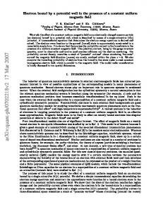
Fig.1 with chromosome lengths of L = 32, 64, 128 and 512 is incomplete. By including a larger length of L = 1024 , one gets Fig.2.
100 L = 32 ... 512
probability density
L = 1024 1
10−2 b = 0.02 P = 10000 10−4 0
0.2
0.4
0.6
genetic load (N/L) Figure 2: The same data displayed in Fig.1, now within a wider horizontal scale in order to fit further data obtained for a larger chromosome length of L = 1024 (rightmost bell shaped curve). The population size is still P = 10000 , the birth/death rate b = 0.02 , and m/L = 1/320 ≈ 0.003 . Unlike the collapsed curves of Fig.1, now repeated at the left-handed side of Fig.2, the larger chromosome length of L = 1024 shows a runaway from the wild-type genotype ( N = 0 ) towards the random situation ( hN i ≈ L/2 ). Beyond this length, the wild-type genotype is extinct and the whole population distribution is no longer glued to it. The same behaviour is also observed in many other similar systems, in particular the pioneering Eigen model [5]. Beyond a certain limit for the chromosome length L , the scaling properties denoted by the collapse of many curves into a single distribution containing the wild-type genotype no longer hold. The preliminary conclusion at the end of last section is now in check. We need a more detailed analysis, which follows. Let’s consider different values for the parameter m , the average number of mutations performed at birth. Fig.3 shows the average genetic load hN i/L as a
6
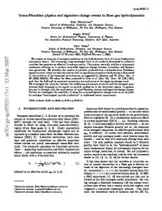
function of m , for various chromosome lengths L = 32, 64, 128 . . . 2048 (black circles) and 4096 (black squares). In the limit of large enough chromosome lengths, this figure seems to display a first order phase transition. The average genetic load vanishes if the number m of mutations remains below a certain threshold mc (here, mc ≈ 3 ). This would be the survival phase, where the population genetic quality is not compromised by too much mutations at birth. On the other hand, for m > mc , one observes the average genetic load suddenly jumping up and approaching the pure random value hN i/L = 0.5 , where no evolution is possible, as explained in the next two paragraphs.
average genetic load (/ L)
0.5
0.25
L = 32, 64 ... 4096 b = 0.02 P = 10000
0 0
2
4
6
mutations per offspring (m) Figure 3: Apparent first order phase transition: survival on the left, extinction on the right. For large enough chromosome lengths, the curve approaches a step. Evolution is possible only below this step, on the left-handed side, where the genetic degradation (as measured by the density of “bad genes” read on the vertical axis) is far below the random behaviour hN i/L ≈ 0.5 . The number m of mutations performed at birth should be smaller than the threshold mc ≈ 3 . Beyond this point, the sudden jump towards the random behaviour forbids evolution to proceed. After the runaway observed in Fig.2 for L = 1024 , the distribution curves for larger and larger values of L (not shown in Fig.2 for clarity) would be sharper and sharper, all of them centred near N/L ≈ 0.5 , reaching N/L = 0.5 for
7
L → ∞ . Therefore, within negligible (sub-linear) fluctuations, all individuals share the same phenotype N ≈ L/2 and become selectively alike to each other. No selection, no evolution. Technically, by putting such a sharp distribution H(N ) in Eq.(1) one gets the solution x = 1 in the limit of large values of L (or N ). However, this solution is a biological nonsense, because it implies eternal survival for all individuals, again no evolution. In reality, for such sharp distributions far from N/L = 0 , the population would undergo a genetic meltdown, and will be eventually extinct. This fate is artificially avoided by our assumption of a constant size population, which no longer holds. We could correct this failure and observe real extinction, simply by imposing some maximum value xmax near but strictly smaller than unity, if the solution x obtained from Eq.(1) surpasses this limit. However, this procedure is unnecessary because we are interested only in the survival which holds on the left-handed side of Fig.3, where always one gets x < 1 from Eq.(1).
average genetic load (/ L)
0.5
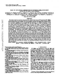
L = 32, 64 ... 4096 b = 0.02 P = 32000 0.25
0 0
2
4
6
mutations per offspring (m) Figure 4: For a larger population of P = 32000 , the apparent transition occurs at a larger threshold mc ≈ 5 , as compared to Fig.3. On the survival side of Fig.3 or Fig.4, the plots correspond to straight lines starting at the origin, whose slopes decrease with increasing L proportionally to 1/L . Thus, by keeping the same ratio m/L for increasing values of L , one
8
gets always the same value for hN i/L read on the vertical axis along a plateau, provided m does not surpass the transition point mc (i.e. provided L is not too large). In reality, not only the average hN i/L , but the whole distribution of N/L does not depend on L , as in Fig.1. Is this phase transition genuine? In order to answer this question, we need to consider the so-called thermodynamic limit (the limit of larger and larger populations) and ask whether the (would-be) phase transition remains. According to traditional statistical physics, phase transitions occur only in this limit. We could, for instance, repeat Fig.1 for a larger population, say P = 32000 . We do not need to show such a plot, because it is the same as Fig.1. The only difference is that L = 1024 now fits into the same collapsed curve shown in Fig.1, instead of following the runaway observed in Fig.2. In fact, the runaway does not occur if the population size is large enough. Fig.4 corresponds to a larger population of P = 32000 , to be compared with the former Fig.3: now, the apparent transition point is located at mc ≈ 5 , larger than the former value.
average genetic load (/ L)
0.5
0.25
0 0
2
4
6
8
10
mutations per offspring (m) Figure 5: The (would-be) transition occurs at different locations for different population sizes P = 1000, 3200, 10000, 32000 and 100000 from left to right. Squares correspond to L = 2048 , and lines to L = 4096 . Fig.5 shows again the average genetic load hN i/L as a function of m , for increasing populations sizes. For clarity, only data corresponding to the two 9
largest chromosome lengths L = 2048 (squares) and 4096 (lines) are shown. The larger the population size, the larger the transition point mc . As an estimate for mc , we have taken the crossings of the L = 4096 curves with the horizontal line hN i/L = 0.25 (just half-way from the complete order N = 0 towards the complete disorder hN i = L/2 ). The resulting values of mc obtained from these crossings are plotted against P in Fig.6. They follow a power-law, and this behaviour indicates that mc grows indefinitely for larger and larger populations. In this limit P → ∞ at fixed m/L , only the survival phase exists, no runaway.
transition point (mc)
10
1 1000
10000
100000
population size (P) Figure 6: The transition point increases for increasing population sizes, following a power-law. The straight line mc ∝ P 0.44 fits very well the data. It means that one needs a minimum population size Pmin ∝ L1/0.44 = L2.3 in order to sustain the population survival at a fixed m/L , where L is the chromosome length. The apparent survival-extinction transition shown in plots like Fig.3 is not a genuine phase transition, it disappears for large enough population sizes. Therefore, the preliminary conclusion we have stated at the end of last section is not completely wrong. Indeed, in order to keep the same genetic quality of the population for increasing chromosome lengths, one should keep the same rate of errors when each chromosome is copied for reproduction, i.e. the same probability of error per locus, m/L . However, this is not a priceless procedure.
10
The population size should also be large enough to avoid the runaway shown in Fig.2. The minimum required population size depends on the largest chromosome length one wants to reach. The current paper deals with asexual populations. In another paper [1] we have shown that this conclusion does not hold for sexually reproducing populations. In this case, the survival-extinction transition is a genuine one, the transition point mc does not depend on the population size. When the chromosome length is increased, one should keep the same absolute number m of mutations performed at birth, not the ratio m/L . Therefore, with sex, the price to pay for increasing the chromosome length is higher: one should improve the performance of the chemical DNA copying machinery, in order to keep the same number of errors, in spite of a larger length to be copied. We close this section with a technical comment on the simulations. The evolutionary time one needs to reach genetic stabilisation is very huge, particularly near the jumps shown in plots like Fig.3, Fig.4 or Fig.5. Starting from an initial population with only N = 0 individuals, one needs to evolve the whole population through 108 or more time steps in order to reach the runaway shown in Fig.2. In order to control the statistics, we simulated a total of 10 independent populations, taking averages at the end, with error bars. For that reason, our computer program runs for a long time in an Athlon/Opteron 250 processor, up to ≈ 10 days for each point shown on the rightmost curve on Fig.5.
11
3
Conclusions
Based on a very simple model which nevertheless contains both fundamental ingredients which drive Darwin’s evolution, namely random mutations performed at birth and natural selection, we have discovered some chromosome length scaling properties. The overall result (valid in the thermodynamic limit) is very simple to state: in order to increase the chromosome length L , one should keep the same mutation rate m/L per locus, where m is the average number of point mutations performed at birth. This result is also in complete agreement with human intuition, since the number m of errors found in a chromosome copy should be proportional to its length L , when performed by the same chemical DNA copying machinery. However, the issue is not so simple, not so intuitive. The validity of this linear behaviour depends on the population size. It should be large enough to avoid the genetic meltdown characterised by the runaway shown in Fig.2, which means extinction. We have also shown that a minimum population size is required to avoid this, which increases for larger and larger chromosome lengths as Pmin ∝ Lα where our numerical estimate for the exponent is α ≈ 2.3 . By including sex with crossings and recombination, another completely different scaling holds, independent of the population size: m instead of m/L should be preserved when a L−scaling transformation is performed [1, 2].
12
References [1] P.M.C. de Oliveira et al, Does Sex Induce a Phase Transition? in preparation (2006). [2] D. Stauffer, S. Moss de Oliveira, P.M.C. de Oliveira and J.S. S´ a Martins, Biology, Sociology, Geology by Computational Physicists, pages 49–69, Elsevier, The Netherlands (2006). [3] P.M.C. de Oliveira, Theory in Biosciences 120, 1 (2001), also in cond-mat 0101170. [4] G. Parisi, Physica A263, 557 (1999). [5] M. Eigen, Naturwissenschften 58, 465 (1971); M. Eigen, J. McCaskill and P. Schuster, Adv. Chem. Phys. 75, 149 (1989).
13


![arXiv:math/0703218v1 [math.NT] 8 Mar 2007](https://m.moam.info/img/260x300/arxivmath-0703218v1-mathnt-8-mar-2007_5ba1fb3e097c47296d8b45f3.jpg)
![arXiv:math/0510359v3 [math.RT] 8 Mar 2007](https://m.moam.info/img/260x300/arxivmath-0510359v3-mathrt-8-mar-2007_5ba704d1097c47d37f8b4575.jpg)
![arXiv:math/0703226v1 [math.PR] 8 Mar 2007](https://m.moam.info/img/260x300/arxivmath-0703226v1-mathpr-8-mar-2007_5a639ece1723dd28be977947.jpg)
![arXiv:math/0703215v1 [math.DS] 8 Mar 2007](https://m.moam.info/img/260x300/arxivmath-0703215v1-mathds-8-mar-2007_5ba27f7e097c475f378b4703.jpg)


![0405030v3 [math.GT] 21 Mar 2007](https://m.moam.info/img/260x300/0405030v3-mathgt-21-mar-2007_5c67933d097c47703d8b4611.jpg)
![0512132v2 [math.NT] 21 Mar 2007](https://m.moam.info/img/260x300/0512132v2-mathnt-21-mar-2007_5c1b7b12097c470f588b45bc.jpg)
![0703173v1 [math.PR] 6 Mar 2007](https://m.moam.info/img/260x300/0703173v1-mathpr-6-mar-2007_5c329287097c471c398b45ba.jpg)
![0606018v2 [math.CO] 15 Mar 2007](https://m.moam.info/img/260x300/0606018v2-mathco-15-mar-2007_5c261c63097c47bf218b4605.jpg)
![0703664v1 [math.RT] 22 Mar 2007](https://m.moam.info/img/260x300/0703664v1-mathrt-22-mar-2007_5c9ceef3097c47011d8b4622.jpg)
![0703417v1 [math.AC] 14 Mar 2007](https://m.moam.info/img/260x300/0703417v1-mathac-14-mar-2007_5c71383f097c47a3718b4632.jpg)
![0608502v2 [math.GM] 21 Mar 2007](https://m.moam.info/img/260x300/0608502v2-mathgm-21-mar-2007_5c438959097c477a1e8b45f5.jpg)
![0703154v1 [math.AC] 6 Mar 2007](https://m.moam.info/img/260x300/0703154v1-mathac-6-mar-2007_5c67b94a097c47f1588b459b.jpg)

![0703687v1 [math.CV] 23 Mar 2007](https://m.moam.info/img/260x300/0703687v1-mathcv-23-mar-2007_5c5cbfc1097c472d308b45ff.jpg)
![0703280v1 [math.CA] 10 Mar 2007](https://m.moam.info/img/260x300/0703280v1-mathca-10-mar-2007_5c288d03097c479f608b4576.jpg)