Rua Sérgio Buarque de Holanda, 777, Cidade Universitária, 13083-859, Campinas, SP, Brasil. Abstract. We determine the Lie point symmetries of a class of ...
Communications in Nonlinear Science and Numerical Simulation Volume 69, April 2019, Pages 73-77. DOI: 10.1016/j.cnsns.2018.09.011
Lie point symmetries and conservation laws for a class of BBM-KdV systems Valter Aparecido Silva Junior a,b a
Instituto Federal de Educa¸c˜ ao, Ciˆencia e Tecnologia de S˜ao Paulo - IFSP. Avenida Marginal, 585, Fazenda Nossa Senhora Aparecida do Jaguari, 13871-298, S˜ao Jo˜ao da Boa Vista, SP, Brasil. b
Instituto de F´ısica “Gleb Wataghin” - IFGW, Universidade Estadual de Campinas - UNICAMP. Rua S´ergio Buarque de Holanda, 777, Cidade Universit´aria, 13083-859, Campinas, SP, Brasil.
Abstract We determine the Lie point symmetries of a class of BBM-KdV systems and establish its nonlinear self-adjointness. We then construct conservation laws via Ibragimov’s Theorem. Keywords: BBM-KdV system, Lie point symmetries, nonlinear self-adjointness, conservation laws.
1
Introduction
Motivated by the works [4, 5], we introduce the following class of systems ( F1 ≡ ut + (a + b)vux + (au + c)vx + �utxx + κvxxx = 0 , F2 ≡ vt + (bu + c)ux + (a + b)vvx + λuxxx + σvtxx = 0
(1)
henceforth simply referred to as BBM-KdV system, a two-component generalization1 of the classic equations [2] BBM: ut + (u + 1)ux − utxx = 0
(2)
KdV : ut + (u + 1)ux + uxxx = 0,
(3)
and with the objective of studying it from the point of view of the group analysis. 1
If u = v, the system (1) is reduced to equations ut + [(2a + b)u + c]ux + �utxx + κuxxx = 0 and ut + [(a + 2b)u + c]ux + σutxx + λuxxx = 0. Both contain (2) and (3) as special cases.
1
In (1), the constants are such that (a + b)c 6= 0 and {�, κ, λ, σ} = 6 {0}. Particularly when a = c = 1 and b = 0, we obtain the already widely investigated systems of Boussinesq (� = κ = λ = 0, σ = −1/3), Kaup (� = λ = σ = 0, κ = 1/3) and BonaSmith (� = σ = λ/2 − 1/6, κ = 0, λ < 0), all of them first-order approximations to the Euler equations in the framework of hydrodynamics. Useful in situations where dissipative effects are not significant, these models provide a good description for the two-dimensional motion of small-amplitude long waves on the surface of an ideal fluid. In this context, the independent variable x represents the distance traveled along a fixed depth channel and t the time. The quantities u(t, x) and v(t, x) are related to the deviation of the surface from its undisturbed level and to the horizontal velocity of the fluid, respectively. For more information, see [4, 5] and references therein. Relevant results, including exact solutions, can be found in [1, 6, 7]. It’s well known that evolution equations don’t possess an usual Lagrangian. Therefore this paper is thus organized: first we determine the Lie point symmetries (Section 2) of the BBM-KdV system and establish its nonlinear self-adjointness (Section 3); we then construct conservation laws via Ibragimov’s Theorem (Section 4), an extension of the celebrated Noether’s Theorem to problems with no variational structure. In the next sections, unless otherwise stated, ci ’s are arbitrary constants. All functions are smooth. We consider that the reader is familiar with the fundamental concepts of group analysis. The basic literature used is [3, 8, 9, 10, 11, 12, 13, 14].
2
Lie Point Symmetries Classification
Without many details, applying the standard algorithm presented in [3] and [14], a differential operator X = T (t, x, u, v)
∂ ∂ ∂ ∂ + X (t, x, u, v) + U(t, x, u, v) + V(t, x, u, v) ∂t ∂x ∂u ∂v
generates the Lie point symmetries of the system (1) if the conditions of invariance (the so-called determining equations) Tx = Tu = Tv = Xu = Xv = 0, �Xt = �Xx = σXt = σXx = 0, Ut = Ux = Uv = Vt = Vx = aU − (au + c)Uu = 0, bU + (bu + c)[Uu + 2(Tt − Xx )] = 0, κ(Uu + 2Xx ) = λ[Uu + 2(Tt − 2Xx )] = 0, (a + b)[V + (Tt − Xx )v] − Xt = 0 are satisfied. From (4), it’s easy to see that T = (a + b)c1 t + c2 , X = (a + b)(c3 x + c4 t) + c5 , U = 2(c3 − c1 )(au + c), V = (a + b)(c3 − c1 )v + c4 2
(4)
with
b(a − b)(c1 − c3 ) = 0, �c3 = �c4 = κ[ac1 − (2a + b)c3 ] = 0, λ[bc1 − (a + 2b)c3 ] = σc3 = σc4 = 0.
Proposition 1. The Lie point symmetries of the BBM-KdV system are summarized in Table 1, where � � ∂ ∂ ∂ X1 = (a + b) t − v − 2(au + c) , ∂t ∂v ∂u � � ∂ ∂ ∂ ∂ +v + 2(au + c) , X2 = , X3 = (a + b) x ∂t ∂x ∂v ∂u ∂ ∂ ∂ X4 = (a + b)t + , X5 = . ∂x ∂v ∂x
{�, σ} = {0} {�, σ} = 6 {0}
a=b
b(a − b) 6= 0
3X1 + X3 X2 , X4 , X5
X 2 , X4 , X5
X1 (κ = λ = 0) X 2 , X5
X2 , X5
b=0 X1 (κ = 0) 2X1 + X3 (λ = 0) X2 , X4 , X5 X1 (κ = 0), X2 , X5
Table 1.
3
Self-Adjointness Classification
To begin with, let u¯ and v¯ be the new dependent variables. The formal Lagrangian of the system (1) is L = u¯F1 + v¯F2 . Calculated the adjoint equations δL F1∗ ≡ − = u¯t + (a + b)v¯ ux + (bu + c)¯ vx + b¯ uvx + �¯ utxx + λ¯ vxxx = 0 δu , F ∗ ≡ − δL = v¯t + (au + c)¯ ux + (a + b)v¯ vx − b¯ uux + κ¯ uxxx + σ¯ vtxx = 0 2 δv where δ/δu and δ/δv are Euler-Lagrange operators, we assume that F1∗ |(¯u,¯v)=(ϕ,ψ) = M F1 + N F2 ,
F2∗ |(¯u,¯v)=(ϕ,ψ) = P F1 + QF2 .
(5)
Here M , N , P and Q is a set of coefficients to be determined and ϕ = ϕ(t, x, u, v),
ψ = ψ(t, x, u, v) 3
(6)
two functions that not vanish simultaneously. As F1∗ |(¯u,¯v)=(ϕ,ψ) = Dt ϕ + (a + b)vDx ϕ + (bu + c)Dx ψ + bϕvx + �Dt Dx2 ϕ + λDx3 ψ and F2∗ |(¯u,¯v)=(ϕ,ψ) = Dt ψ + (au + c)Dx ϕ + (a + b)vDx ψ − bϕux + κDx3 ϕ + σDt Dx2 ψ, from (5) it’s possible to conclude that M = ϕu , N = ϕv , P = ψu , Q = ψv and ϕt + (a + b)vϕx = �ϕx = 0, ψt + (au + c)ϕx = ψx = 0, bϕ = (au + c)ϕu − (bu + c)ψv , ϕv − ψu = (� − σ)ϕv = κϕu − λψv = 0, �ϕuu = ϕuv = ϕvv = 0. Hence ϕ = (c1 t + c2 )av + f (u) − c1 x, with
ψ = c3 v + (c1 t + c2 )au + c1 ct + c4
bc1 = bc2 = �c1 = σc1 = (� − σ)c2 = 0, �f 00 (u) = κf 0 (u) − λc3 = 0, bf (u) = (au + c)f 0 (u) − (bu + c)c3 .
Proposition 2. The BBM-KdV system is nonlinearly self-adjoint. The substitutions (6) are as follows. i) If b = 0, ϕ = (c1 t + c2 )av + c3 c ln(au + c) − c1 x + c4 , where
ψ = c3 av + (c1 t + c2 )(au + c) + c5
6 {0}, c1 = 0, to {�, σ} = c2 = 0, to � 6= σ, c3 = 0, to {�, κ, λ} = 6 {0}.
ii) If a = b, ϕ = (au + c)[c1 ln(au + c) + c2 ], where
(
ψ = c1 av + c3
c1 = 0, to {�, κ, λ} = 6 {0}, c2 = 0, to κ 6= 0.
iii) Let b(a − b) 6= 0. 4
iii.a) If a = 0, ϕ = c1 ebu/c − c2 (bu + 2c), where
(
ψ = c2 bv + c3
c1 = 0, to {�, κ} = 6 {0}, c2 = 0, to κ 6= −λ.
iii.b) If a 6= 0, ϕ = c1 (au + c)b/a + c2 [b2 u + (2b − a)c], where
(
ψ = c2 (a − b)bv + c3
c1 = 0, to {�, κ} = 6 {0}, c2 = 0, to λa 6= (κ + λ)b.
Remark. Actually, the system (1) is quasi self-adjoint. It becomes strictly self-adjoint in only two circumstances: a = 2b and κ = λ; or b = 0 and � = σ.
4
Conservation Laws
In view of Proposition 2, the components of the conserved vector C = (C t , C x ) associated to X, a Lie point symmetry admitted by the system (1), are according to Ibragimov’s Theorem given by C t = (ϕ − �Dx ϕDx )W u + (ψ − σDx ψDx )W v and C x = [(a + b)vϕ + (bu + c)ψ + �(ϕDt Dx + Dt Dx ϕ) + λ(ψDx2 − Dx ψDx + Dx2 ψ)]W u + + [(au + c)ϕ + (a + b)vψ + σ(ψDt Dx + Dt Dx ψ) + κ(ϕDx2 − Dx ϕDx + Dx2 ϕ)]W v , with W u = U − T ut − X ux ,
W v = V − T vt − X vx .
We find the conservation laws corresponding to each generator of Table 1. In most cases, however, we are led to trivial vectors or the vectors C t = u + �uxx ,
C x = (au + c)v + κvxx
and C t = 2(v + σvxx ),
C x = (a + b)v 2 + (bu + 2c)u + 2λuxx
that can be obtained from the first (when b = 0) and second equation of the BBM-KdV system by simple integration (obvious conservation laws). The really interesting cases we list below. 5
Proposition 3. i) Let b = 0. i.a) From X1 , 2X1 + X3 and X2 , we obtain C t = 2(uv − �ux vx ), C x = cu2 + (2au + c)v 2 − (λu2x + κvx2 ) + 2[u(λux + �vt )x + v(�ut + κvx )x ] when � = σ. i.b) For � = κ = 0, X1 also provides 1 a C t = (au + c) ln(au + c) + (v 2 − σvx2 ), a 2c � � av av 2 x C = (au + c)[ln(au + c) + 1]v + + σvtx c 3 when λ = 0 and C t = 2[t(au + c)v − xu], C x = t[c(au + 2c)u − aλu2x ] + 2(au + c)[(atv − x)v + λtuxx ] when σ = 0. ii) Let a = b. ii.a) From X1 and 3X1 + X3 , we obtain C t = (au + 2c)u − a�u2x , C x = 2(au + c)[(au + c)v + �utx ] when κ = 0. ii.b) X1 also provides 1 C t = (au + c)2 ln(au + c) + a(v 2 − σvx2 ), a � � 2av 2 x 2 C = (au + c) [2 ln(au + c) + 1]v + 2av + σvtx 3 when � = κ = λ = 0.
6
References [1] Antonopoulos DC, Dougalis VA, Mitsotakis DE. Numerical solution of Boussinesq systems of the Bona–Smith family. Appl Numer Math 2010;60:314–36. [2] Benjamin TB, Bona JL, Mahony JJ. Model equations for long waves in nonlinear dispersive systems. Phil Trans R Soc Lond A 1972;272:47–78. [3] Bluman GW, Kumei S. Symmetries and differential equations. New York: Springer; 1989. [4] Bona JL, Chen M, Saut JC. Boussinesq equations and other systems for small– amplitude long waves in nonlinear dispersive media. I: Derivation and linear theory. J Nonlinear Sci 2002;12:283–318. [5] Bona JL, Chen M, Saut JC. Boussinesq equations and other systems for small– amplitude long waves in nonlinear dispersive media: II. The nonlinear theory. Nonlinearity 2004;17:925–52. [6] Chen M. Exact solutions of various Boussinesq systems. Appl Math Lett 1998;11:45–9. [7] Dougalis VA, Duran A, Lopez–Marcos MA, Mitsotakis DE. A numerical study of the stability of solitary waves of the Bona–Smith family of Boussinesq systems. J Nonlinear Sci 2007;17:569–607. [8] Gandarias ML. Weak self–adjoint differential equations. J Phys A Math Theor 2011;44:262001 (6 pp). [9] Ibragimov NH. Integrating factors, adjoint equations and Lagrangians. J Math Anal Appl 2006;318:742–57. [10] Ibragimov NH. A new conservation theorem. J Math Anal Appl 2007;333:311–28. [11] Ibragimov NH. Quasi–self–adjoint differential equations. Arch Alga 2007;4:55–60. [12] Ibragimov NH. Nonlinear self–adjointness and conservation laws. J Phys A Math Theor 2011;44:432002 (8 pp). [13] Ibragimov NH. Nonlinear self–adjointness in constructing conservation laws. Arch Alga 2011;7/8:1–90. [14] Olver PJ. Applications of Lie groups to differential equations. New York: Springer; 1986.
7