(TOC), acquisition cost, airframe manufacturer's cash flow, and airline's return on investment. The assessment of these criteria was performed through the ...
PRELIMINARY ASSESSMENT OF THE ECONOMIC VIABILITY OF A FAMILY OF VERY LARGE TRANSPORT CONFIGURATIONS
Dr. Dimitri N. Mavris Assistant Professor & Manager, ASDL
Michelle R. Kirby Graduate Student Research Assistant, ASDL
Aerospace Systems Design Laboratory School of Aerospace Engineering Georgia Institute of Technology Atlanta, Georgia 30332-0150
ABSTRACT
INTRODUCTION
A family of Very Large Transport (VLT) concepts were studied as an implementation of the affordability aspects of the Robust Design Simulation (RDS) methodology which is based on the Integrated Product and Process Development (IPPD) initiative that is sweeping through industry. The VLT is envisioned to be a high capacity (600 to 1000 passengers), long range (~7500 nm), subsonic transport. Various configurations with different levels of technology were compared, based on affordability issues, to a Boeing 747-400 which is a current high capacity, long range transport. The varying technology levels prompted a need for an integration of a sizing/synthesis (FLOPS) code with an economics package (ALCCA). The integration enables a direct evaluation of the added technology on a configuration economic viability. The determination of the viability was based on the assessment of the following evaluation criteria: average yield per Revenue Passenger Mile ($/RPM), Total Operating Cost per day (TOC), acquisition cost, airframe manufacturer's cash flow, and airline’s return on investment. The assessment of these criteria was performed through the application of several statistical techniques such as Response Surface Methodology (RSM), Design of Experiments (DoE), and Monte Carlo Simulations. The result is a series of second-order equations that model the evaluation criteria above stated. The final conclusion of this analysis is that the 800 passenger configuration would meet most of the market demand (600 to 1600 passengers) of 250 city pairs considered. This paper reviews the RDS methodology and how it was applied to determine the economic viability of a VLT concept. In addition, it documents the results of the method used to determine the economic viability of a family of VLT configurations and the most affordable VLT configuration for a specified market demand.
Despite the fact that in recent years, airlines worldwide have experienced numerous financial difficulties, many feel that the need for long range business travel may be declining in the era of satellite communications, computer networking, and electronic mail. Recent surveys predict that air travel will double by the year 2005. This predicted growth is anticipated to be especially large in the Asian-Pacific markets, where economic analysts predict this region to be the air transport market for the next twenty years. This potential increase in traffic is expected to strain the existing infrastructures causing a need for considerable expansion of existing airports or construction of new ones. Either alternative is considered extremely expensive or impractical and does not answer the increased congestion problem. Another option is a high capacity, long range aircraft which can meet the increased travel demand as well as maximize landing and takeoff slot utilization at existing airports1. In a recent Airbus survey2, 12 airlines from Europe, the U.S., and the Asian-Pacific region expressed a future need for an airplane much larger than the B747-400, that is, between 600 and 1000 passengers. In fact, Upali Wickrama, the chief of forecasting and economic planning for the International Civil Aviation Organization, predicts that by the year 2015 there will be a demand for an additional 443 aircraft with 400-600 seats and 360 aircraft with greater than 600 seats3. Though these studies favorably show the need for a VLT, another prediction that deserves considerable attention is that air travel is expected to move from the business market to the more price sensitive tourist market. Since tourism is focused more on ‘luxury’ than business travel, tourists will only be willing to travel abroad if it is affordable and comfortable. Consequently, airlines are looking for a 600 to a 1000 passenger airplane with an affordable ticket price for the passenger while maintaining a reasonable Return On Investment (ROI). As a result, the following goals were established for the development of the VLT concept:
Paper presented at the 1st World Aviation Congress, Los Angeles, CA, October 22-24, 1996 Copyright © 1996 by the American Institute of Aeronautics and Astronautics, Inc. All rights reserved.
1
1. 2. 3. 4. 5.
Achieve at least a 30% reduction in passenger ticket fare as compared to the Boeing 747-400; Achieve a high ROI for the airlines; Achieve a low aircraft unit cost to reduce the risk of investment for the airlines; Minimize the number of aircraft required to meet the predicted market demand needs; and Determine the appropriate size (i.e., number of passengers) for further study of the VLT concept.
The response to these goals was the focus of this study. IMPLEMENTATION The Aerospace industry is shifting its focus from design for performance to that for affordability. This trend may be viewed as a direct result of budget restrictions and increasing aircraft systems costs. Therefore, a need exists for the development of an approach which counteracts these effects through the implementation of techniques and methodologies that consider the entire design and life-cycle of an aircraft. The Robust Design Simulation (RDS) is such a technique and is based on the Integrated Product and Process Development (IPPD) initiative that is sweeping through industry. The RDS methodology extends traditional single objective optimization approaches to one based on an overall perspective of achieving customer satisfaction. In this case, customer satisfaction, may be defined as life-cycle cost reduction, improved reliability, manufacturer’s Return on Investment, etc. RDS provides a systematic approach which may be used to find the optimal design factor settings which result in economic designs with low variability. RDS is applicable to many design situations, but it will be used to assess the demands stated previously. The RDS implementation procedure followed to address the economic variability in the presence of uncertainty for a generic VLT configuration is shown in Figure 1. Statistical approaches, such as the Response Surface Methodology (RSM)4,5, Design of Experiments (DoE)5,6 and Monte Carlo simulations7,8 are incorporated into the procedure, as described in detail in Ref. 9. For vehicle sizing and synthesis, the Flight Optimization System code, FLOPS10, is used to translate mission requirements, design variables, and constraints at a given level of technology into an aircraft configuration. The geometric, weight, and propulsion characteristics of this vehicle are then passed on to the Aircraft Life Cycle Cost Analysis, ALCCA11, module to complete the economic assessment. ALCCA is comprised of a series of modules capable of predicting aircraft acquisition cost, Return on Investment (ROI) for the airline and manufacturer, cash flows, etc. The original stand-alone version was integrated into FLOPS so that immediate knowledge of the affordability aspects, as affected by the various designs, can be determined. Through the application of a DoE approach, an analysis of variance is performed to determine a suitable polynomial equation which can represent a chosen response. This response will be a function of the most significant economic variables based on a Pareto analysis performed on the results obtained from ALCCA. For the cases described in this paper, the
response, R, was found to behave as a second-order polynomial. This so called Response Surface Equation (RSE) can be described by an equation of the form: k
k
k
i =1
i =1
i =1
R = bo + ∑ bi xi + ∑ bii xi2 + ∑ ∑ bij xi x j
(1)
where: the bi represent the regression coefficients for the linear terms; b ii the quadratic coefficients; b ij the cross-product coefficients (i.e. second-order interactions); x i, x j the design variables; and x ix j denotes interactions between two design variables. Once EQ (1) is determined, it can be used in lieu of more sophisticated, time consuming codes to predict and optimize the response of a sub-system or the entire system. The “optimal” settings for the design variables can then be identified by finding the maximum or minimum of this equation. In the case of a commercial transport, the most suitable overall evaluation criterion with respect to affordability was found to be the average yield per Revenue Passenger Mile ($/RPM). This metric implicitly captures the concerns and interests of the airline, manufacturer, and passenger. The airline and manufacturer interests, represented by profitability, are measured in terms of Return on Investment (ROI) while the passengers are interested in an affordable ticket price. Mission Requirements
Design Variables
Vehicle Sizing and Synthesis
Infusion of New Technology
FLOPS
Mission, Design Constraints
Configuration Description
JMP DOE
Manufacturing Considerations ALCCA
Economic Assumptions
Market/Airline Concerns Response RSM-Equation Critical Technology Identification
Crystal Ball Monte Carlo Simulation
Economic Uncertainty
Response Probability Distribution
Yes
Improvement possible ?
No
Terminate Program
No
Economic Viability
Yes
Launch Program
Figure 1: RDS Implementation Procedure At this time, economic uncertainty is introduced into the design. A Monte Carlo Simulation is performed with the aid of a software package called Crystal Ball6. Crystal Ball generates values randomly for the most significant variables based on user-specified probability distributions. These are used to compute the overall probability distribution for the 2
given response. The resulting distribution of $/RPM yields a feasible design which is then tested to determine whether it is also economically viable. If the Monte Carlo Simulation identifies a non-viable solution, areas of possible technology improvement must be identified and evaluated. If no improvement is possible, or the alternatives are simply too risky from a schedule or budget viewpoint, then early program termination is recommended before more resources are expended. APPROACH The study presented here attempts to recognize and identify the proper size vehicle, that is, the number of passengers and the right blend of technologies which will yield an economically viable configuration. The combined RSM/Monte Carlo analysis was applied to a family of VLT configurations so that their economic uncertainty could be quantified. The VLT initiative is currently in the concept feasibility stages of its development and is envisioned to be a double-decker, subsonic aircraft capable of carrying 600 to a 1000 passengers to destinations in excess of 7500 nautical miles. The present focus is to determine which configuration, 600, 800, or 1000 passengers, is most suitable for the market growth predicted over the next 10 to 15 years. In order for a concept such as the proposed VLT to be produced, it must abide by existing FAR and EPA regulations, be comparable in safety and comfort to the current long range subsonic fleets, and provide economic benefits to all interested parties, i.e., manufacturer, airline, and passenger. Therefore, it is essential to maintain an affordable ticket fare for the passenger while retaining a reasonable ROI for both the airline and the airframe/engine manufacturers. Thus, the overall objective is to achieve a robust design that meets the target value set for the criteria function. For this study, the $/RPM target, as stated previously, is based on an approximate 30% fare reduction in ticket price with respect to large subsonic transports similar in size to the Boeing 747-400. The exact value of this target was established by applying the RDS to the B747-400 configuration with the same ground rules and assumptions used for the various VLT alternative configurations. The economics, i.e., $/RPM, acquisition costs, etc., were established through the use of the integrated FLOPS/ALCCA code. Note that the economic figures obtained for the baseline configuration target do not match the actual numbers of the current B747-400 (as developed in the 1960s) due to the assumption that the aircraft was evaluated as if it was a hypothetically new program launched today. DEVELOPMENT OF AIRCRAFT CONFIGURATIONS Baseline VLT configurations are based on work performed by Dennis Bartlett, et. al., at NASA Langley Research Center12. There are three baseline configurations (600, 800, and 1000 passengers) with various levels of technology depicted in Table I. These technology levels allowed for eight permutations per aircraft configuration. The configurations from this point on will be referred to as the V600, V800, or
V1000 based on how many passengers they carry (600, 800, or 1000 passengers respectively). The configurations were sized by FLOPS with an engine technology level representative of a 1995 entry into service and a typical commercial subsonic mission. The ground rules and assumptions associated with the FLOPS synthesis are described in Table II. Table I: VLT Configurations Description Level of Technology
Description of Technology Added
Baseline
Conventional configuration with a wing Aspect Ratio (AR) = 11 Supercritical composite wing with AR = 11 Supercritical composite wing with AR = 11 and Hybrid Laminar Flow Control (HLFC) Supercritical composite wing with AR = 11, HLFC, and composite fuselage
Highest Level
All aircraft configurations conformed to these guidelines with additional constraints imposed upon the fuselage length and diameter. The V600, V800, and V1000 lengths and diameters for a typical dual-class seating arrangement were 230/23.63, 250/27, and 295/27 feet, respectively. The V1000 was identical to the V800 configuration with the exception that two 22.5 ft. plugs were added forward and aft of the wing/fuselage juncture. The sized aircraft were compared to the work performed by Bartlett, et. al.,12 and were confirmed within an error less than 1% for all output parameters, e.g. take-off gross weight, operating empty weight, mission fuel, etc. Table II: Ground Rules and Assumptions for VLT Configuration Sizing Parameter Cruise Mach Number Range Cruise Altitude Wing Loading Thrust-to-Weight Ratio HT Volume Coefficient VT Volume Coefficient Approach Speed Take Off Field Length Maximum Thrust per Engine Nacelle Length Nacelle Diameter Passenger/Baggage
Value 0.85 7500 39,000 154 0.257 1.026 0.071 150 11,000 78,000 22.2 13.77 209
Unit nm ft lb/ft2
kts ft lb ft ft lb
UNCERTAINTY ASSESSMENT FOR THE VLT FAMILY The first step in an economic uncertainty assessment is the identification of all pertinent cost parameters. Figure 2 depicts the majority of the contributors in a cause and effect diagram. All of these parameters are inputs to ALCCA and may be selected for the economic assessment study. The Ishikawa13 diagram displayed presents the various design and cost variables which affect the overall criterion, $/RPM. The diagram is from an airline’s point of view; that is, all of the economic variables above the horizontal vector leading to the $/RPM refer to the airline revenue, while all entities below the vector correspond to expenditures. 3
Screening Test The second step of this economic uncertainty study was the development of an equation for the response of interest in terms of the key economic variables. Based on a Pareto analysis14, a screening test was conducted using a two-level DoE linear model (two extreme points plus a center point) in order to reduce the number of cases that had to be performed in order to develop the RSE. After obtaining the response outputs from FLOPS/ALCCA, an Analysis of Variance, ANOVA14, for only the main effects was performed to obtain each variable’s contribution. A Pareto plot, Figure 3, displays these contributions for the V800 configuration. Figure 3 was generated with the help of a statistical analysis package, JMP15. The relative influence of each variable is given by the depicted bars, while the solid curve represents their cumulative contribution to the response. Table IV: Economic Ground Rules and Assumptions Performance
Weights/ Interior/ Crew
Figure 2: Ishikawa Diagram Through a brainstorming exercise, the ranges for these significant variables were established and are presented for review in Table III. These values were input into FLOPS/ALCCA in accordance with a DoE table for the screening test and the Box-Behnken6 format for the RSE development. The ground rules and assumptions agreed on for the economic uncertainty analysis are given in Table IV. Table III: Economic Input Variables and Their Settings Variable Composite Wing (CompW) Composite Fuselage (CompF) HLFC ROI - Airline (ROIa) ROI - Manufacturer (ROIm) Economic Range (Econ R) Fuel Cost (Fuel $) Insurance (Ins) Labor Rate (LR) Load Factor (LF) Maintenance Factor (Main) Learning Curve (LC) Mean Time Btwn Failures (MTBF) Production Quantity (Q) Production Rate (Q Rate) Utilization (U) Reservations and Sales (R&S)
Minimum No No No 5% 10% 2500 nm $0.54/gal 0.5% of acq cost 100% * 45% 90% 78% 10000 hr
Maximum Yes Yes Yes 15% 20% 7500 nm $0.88/gal 1.0% of acq cost 120% 85% 110% 88% 20000 hr
300 8 years 4500 hr/yr 90%
798 12 years 5500 hr/yr 120%
* 100% refers to present day levels
Spares Rates
Financing Depreciation
Max cruising altitude of 39,000 ft 100% Learning Curve for propulsion system Four engines per aircraft Thrust-to-weight ratio fixed at 0.257 Wing Loading fixed at 154.0 lb/ft2 4 person crew Coach passenger / flight attendant is 26 First class passenger / flight attendant is 12 Aircraft weights based on synthesis analysis Airframe - 6% of total airframe price Propulsion - 23% of total engine price Labor rates of $19.50, $55, and $65 for maintenance, tooling, and engineering, respectively Tax rate of 34% Inflation rate of 8% 100% at 8% interest rate 0% down payment 20 year term 20 years; 10% residual
For this study, the penalty in both development costs and technology risk for advanced technologies was not quantified. Therefore, the effect of introducing new technologies was masked in the screening test by the dominance of the economic uncertainty variables. Therefore, another DoE was applied that optimized the $/RPM based exclusively on the level of technology for a given configuration. Hence, a two-level DoE was performed on each configuration (i.e., V600, V800, and V1000) to determine the level of technology required to minimize the $/RPM. It was determined from this DoE that the highest level of technology was required to minimize $/RPM, acquisition cost, and total operating costs for the different configurations. The results are presented in Table V. The improvement from the baseline to the highest level of technology, as defined in Table I, was roughly 52.9-54.1% in $/RPM. Hence, each configuration baseline contained a supercritical composite wing with AR=11, composite fuselage, and HLFC. Note that only the benefits of advanced technologies are considered here and the risk associated with these technologies will be the focus of future studies.
Term LF ROIa LC Fuel$ U Econ R Q ROIm CompF HLFC CompW LR Ins Q Rate R&S MTBF Main
Scaled Estimate -0.0103823 0.00755044 0.00623200 0.00412296 -0.0027286 0.00230470 0.00226089 -0.0020869 0.00195959 -0.0014639 0.00122209 0.00084346 0.00066122 0.00034184 0.00026596 -0.0002522 0.00008948
.2
.4
.6
RSE for the V800. The RSEs generated for the V600, V1000, and B747-400 are similar in form. The columns presented correspond to the coefficient notation described in EQ (1). The actual equation can now be obtained by the summation of the intercept and all parameter estimates multiplied by their according variable(s).
.8
MANUFACTURER AND AIRLINE ECONOMIC ASSESSMENT
Figure 3: Screening of Main Effects for $/RPM for the V800 at the Highest Level of Technology Table V: Conventional versus Advanced Configurations V600
V800
V1000
$/RPM Acquisition $M $/Trip (design) $/Trip (economic) $/RPM Acquisition $M $/Trip (design) $/Trip (economic) $/RPM Acquisition $M $/Trip (design) $/Trip (economic)
Conventional 0.162 231 528,000 340,400 0.155 285 675,900 435,800 0.153 345 832,700 537,000
Advanced 0.076 174 242,500 158,700 0.073 208 307,400 201,200 0.070 247 374,500 245,000
%∆ -53 -25 -54 -53 -53 -27 -57 -54 -54 -29 -55 -54
Based on the Pareto plot from Figure 3 and the results from the technology DoE, seven highest contributing variables were identified and selected to model the $/RPM. Those seven variables were identified as: load factor, ROI for the airline, learning curve for the manufacturer, fuel cost, utilization, economic range, and production quantity. As indicated in Fig. 3, these variables constitute approximately 80% of the response. The remainder of the variables were fixed at the most likely value or, as in the case of the levels of technology, set at the highest levels. Response Surface Equation Evaluation The surviving independent variables described previously were used to form the Response Surface Equation (RSE) for $/RPM. The RSE was generated using a three-level BoxBehnken design. A Summary of Fit, such as R 2, analysis was employed to ensure that the model fit was acceptable. Modeling fidelity estimates the amount of variation in the response around the mean which is predicted by the fitted model11. The “experiments” performed are computer simulations and are, by definition, 100% repeatable. Therefore, fit error, in this case, is only due to lack of model fit or model error and not to experimental/repetition error. As a general rule of thumb, an R 2 value greater than 90% represents a good model fit8. An R 2 value greater than 99.9% was achieved for the B747-400 and all three VLT configurations. Since this R2 value is close to one, it can be assumed that no higher interactions are significant to the response; therefore, the quadratic representation of the response is a sufficient estimate. Table VI displays the coefficients obtained for the $/RPM
Once the RSEs were determined, an economic analysis probing the manufacturer and airline viability decision making criteria was performed. In fact, the analysis reviewed the impact on manufacturer’s profitability, cashflow, break-even point, ROI, and acquisition cost and price. The ROI for the airline, as well as the Total Operating Cost per trip and per day for the fleet were analyzed. For this study, a FLOPS/ALCCA case was performed with all seven economic variables set at their most likely values and pertinent information was extracted with regards to the above described metrics. Table VI: Response Surface Equation Coefficients for $/RPM for the V800 RSE Coef. b0 b1 b2 b3 b4 b5 b6 b7 b11 b21 b22 b31 b32 b33 b41 b42 b43 b44
Term
Estimate
Intercept 0.326 ROI-A -0.0013 Fuel$ 0.0278 Q -4.8E-05 LF -0.0011 U 3.4E-07 Econ R -5.0E-06 LC -0.0051 ROI-A*ROI-A 2.28E-05 Fuel$*ROI-A 9.27E-05 Fuel$*Fuel$ 0.0011 Q*ROI-A -6.91E-07 Q*Fuel$ 9.0E-07 Q*Q 2.76E-08 LF*ROI-A -1.90E-05 LF*Fuel$ -1.89E-04 LF*Q 2.0E-07 LF*LF 1.18E-05
RSE Coef. b51 b52 b53 b54 b55 b61 b62 b63 b64 b65 b66 b71 b72 b73 b74 b75 b76 b77
Term
Estimate
U*ROI-A U*Fuel$ U*Q U*LF U*U EconR*ROI-A EconR*Fuel$ EconR*Q EconR*LF EconR*U EconR*EconR LC*ROI-A LC*Fuel$ LC*Q LC*LF LC*U LC*EconR LC*LC
-2.23E-07 6.00E-07 2.49E-09 5.69E-08 4.82E-10 -3.79E-09 2.00E-07 1.34E-10 1.59E-08 -5.67E-11 2.59E-10 5.58E-05 -0.00012 -1.67E-07 -0.000016 -1.76E-07 -6.52E-09 0.000046
Manufacturer Items such as cash flow, unit costs (as a function of production size), ROI, and profitability are all key criteria/metrics for the manufacturer. These concerns are functions of parameters such as the type of aircraft, the number of years of production, the levels of technology, and learning curves. The manufacturer’s cumulative net cash flow for the three VLT concepts based on a 12% ROI for the manufacturer are shown in Figure 4. The cash flow is determined by the net income minus the sum of the Research, Development, Testing, and Evaluation (RDT&E), manufacturing, and sustaining costs. The V1000 is the most demanding on the manufacturer with regards to upfront investment for a production run of 10 years starting in 2004. At the most extreme cash flow point, the V1000 represents a 29.4% and 15.4% greater investment than the V600 and V800, 5
aircraft price would be (in FY92 $M) $174.0, $208.5, and $247.0 for the V600, V800, and V1000, respectively. The manufacturer’s profitability for a given aircraft price is shown in Figure 7. The profitability is simply the net cumulative cash flow for the given production run at a given selling price. The manufacturer will have to estimate how much the airlines are willing to invest by means of market outlooks or going aircraft prices as a function of size/weight, etc. Then, the manufacturer must determine how profitable this investment will be at this price. 50 45 ROI-Manufacturer (%)
respectively. Yet, the V1000 generates 29.6% and 15.6% more profit than the V600 and V800 for the same number of aircraft produced (549). The manufacturer is also concerned with the cost of production as affected by the number of aircraft produced. Typically as the number of aircraft produced increases, the cost per unit will decrease as dictated by the learning curve. The unit cost comparisons of the three VLT concepts are shown in Figure 5. These average unit costs are the summation of the component costs of the airframe, propulsion, avionics and instrumentation, and final assembly16. These costs do not include the RDT&E nor the sustaining costs of manufacturing. As is evident from Figure 5, the increased V1000 price might prove to be too expensive of a proposition for the struggling airlines. This higher cost is due to the fact that most of the structural component cost equations are weight-based and the V1000 (1,127,443 lbs) is heavier than the V800 (913,224 lbs) and V600 (716,200 lbs) respectively. 20000
40 35 B747 V600 V800 V1000
30 25 20 15 10 5 0
15000
100
150
200 250 300 Aircraft Unit Price ($M)
Cost (M$ FY92)
10000 5000 0 2004 -5000
350
400
Income
Figure 6: Manufacturer’s Return on Investment 2005
2006
2007
2008
2009
2010
2011
2012
2013
Net Cashflow
80,000 -10000
V600
70,000
V800
-15000
V1000
60,000
Profit ($M)
-20000
Year of Production
Figure 4: Manufacturer’s Cumulative Cash Flow
50,000 B747
40,000
V600 30,000
V800 V1000
20,000
Average Unit Production Cost (M$ FY92)
700
10,000
600
V600
500
V800
400
V1000
0 100
150
200
250
300
350
400
Aircraft Unit Price ($M)
Figure 7: Manufacturer’s Profitability
300 200 100 0 1
10
100
1000
Aircraft Units Produced
Figure 5: VLT Aircraft Unit Production Cost The manufacturer’s ROI is calculated in ALCCA based on the discounted present value of the cumulative net cash flow. Once the period of investment is set, in this case 15 years, the discounted ROI can be determined iteratively when the cash flow is equal to zero. The ROI for the manufacturer increases as the price of the aircraft increases as shown in Figure 6. The V600 can make a reasonable ROI at a lower aircraft price due to the lower unit costs. Furthermore, for the manufacturer to make a 12% ROI for each VLT configuration, the resulting
The manufacturers are also concerned with Life Cycle Costs (LCC). LCC has three main components: RDT&E, production, and Operation and Support (O&S). The relative influence of these three components to the LCC of the 800 passenger configuration is shown in Figure 8. The percentages depicted were found to be of the same order of magnitude for all configurations, thus, only one set of percentages is shown. RDT&E 6% Operations and Support 36% Production 58%
Figure 8: Total Program Costs
6
B747-400, V600, V800, and V1000 would be in FY92 $M, $40.0, $228.5, $317.4, and $396.7, respectively. As can be seen in Fig. 7, the B747 is not competitive with the other aircraft for this $/RPM level. The manufacturer would simply not make a profit; therefore, the airline would not be able to achieve a 12% ROI for a $/RPM of $0.085. B747 V600 V800 V1000
25
20 ROI-Airline (%)
The cost breakdown for each of the primary cost components: RDT&E, production, and O&S, is shown in Figure 9. Within RDT&E, the largest contributor is development support which includes such items as ground test vehicles and spares, flight test operations and spares, and tooling equipment. These costs support the flight test and certification stages of a program. Within the production cost breakdown, the largest contributor, as to be expected, is the cost to build 549 operational vehicles, i.e., those aircraft that are sold to the airlines. This contributor, constitutes the largest expense to a manufacturer. With regards to airline’s O&S costs, the indirect operating costs constitutes the largest percentage. A further cost breakdown of the O&S components: Direct Operating Cost (DOC) and Indirect Operating Cost (IOC), is shown in Figure 10. The largest cost within DOC is flying operations and includes such expenses as flight crew, fuel and oil. Within IOC, the largest expense is passenger service which includes such items as cabin crew service, food and beverage service, and reservation services.
15
10
5
0 0
50
100
150
200
250
300
350
400
Aircraft Price (M$ FY92)
Figure 11: One-to-One Comparison for a $/RPM = 0.085 VARIABILITY ASSESSMENT
Airframe 24%
Ground Support Misc. Support 10% 2% 35% Sustaining 11% Subsystems 9% Spares Avionics Propulsion 10% 8% 24% Operational Vehicles 67% RDT&E
Production DOC 45%
IOC 55%
Operation & Support
Figure 9: RDT&E, Production, and O&S Breakdown
Investment 38%
Flight Oper. 44%
Maintenance 18%
Maintenance System Overhead 8% 12% Aircraft 2% Traffic 8%
Passenger 70%
Introducing economic uncertainty can be easily assessed using the RSE. The uncertainty assessment was performed through a Monte Carlo simulation. Ranges for the variables of the RSE had to be identified. Each variable was assigned a probability distribution over the ranges specified in Table III. A triangular-shaped function distribution was assumed for each variable with the mean at the most likely value. After assigning distributions to the economic variables, the random number generator in Crystal Ball generated values for the independent variables based on the associated distributions. Crystal Ball then used those values to determine the $/RPM value through the RSE. This procedure was repeated 10,000 times to obtain the cumulative probability distributions shown in Figure 12 for each aircraft configuration (i.e. B747-400, V600, V800, and V1000). The cumulative distribution displays the probability/confidence of achieving values less than or greater than a given amount7. That is, if one wants to guarantee a 75% probability that a desired $/RPM will be achieved, then he/she should enter these charts at the .75 probability line and read off the associated $/RPM. A cumulative plot is the most visual means, as compared to a frequency distribution, of determining if a desired confidence level was achieved. B747-400
V600
IOC
1.00
Probability
DOC
Probability
1.00 .75 .50 .25 .00
Figure 10: Direct and Indirect Operating Cost Breakdown
.75 .50 .25 .00
0.04
0.07
0.10
0.13
0.16
0.06
0.07
V800
0.10
0.08
0.09
1.00
.75
Probability
From the airline’s point of view, major items of concern are the $/RPM, ROI, operating, and acquisition cost. Consider a one-to- one comparison shown in Figure 11 with the $/RPM fixed at $0.085. If the manufacturer was to guarantee the airlines a 12% ROI, the resulting acquisition cost for the
0.09
V1000
1.00
Probability
Airlines
0.08
.50 .25 .00
.75 .50 .25 .00
0.06
0.07
0.08
0.09
0.09
0.05
0.06
0.07
Figure 12: Cumulative Function for $/RPM 7
MARKET DEMAND An evaluation of the results depicted in Figure 12 indicate that all VLT configurations meet the desired target of 30% reduction in passenger ticket fare as compared to the B747-400. The B747-400 yielded a 75% confidence of achieving $0.121/RPM while the V600, V800, and V1000 yielded a $0.083, $0.0825, and a $0.073 respectively. At the outset, seven economic variables were chosen to represent the terms in the desired response surface equation of $/RPM. One of those seven variables was the load factor. The range for this variable was between 45% and 85% and was applied to all configuration RSEs. This assumption proved to be invalid when considering a fixed load factor for various passenger capacity aircraft. For example, if a load factor of 50% is assumed for each configuration and the number of passengers on each aircraft determined, the actual number of passengers would vary depending on which configuration was of interest. A B747-400 would have 206 passengers while the V600, V800, and V1000 configurations would have 300, 400, and 500 passengers respectively. Therefore, a re-evaluation based on the market demand, i.e., the number of passengers that would fly a given route, was performed. The market demand was established by evaluating potential markets. The potential markets for the VLT can be divided into two major divisions based on aircraft function: long range and regional. The long range operations are primarily inter-continental and the regional operations would include such city pairs as Narita and Haneda in Japan12. A study of the most likely city pairs for the VLT within these markets was performed. The top 250 city pairs were considered based on distance, number of departures per day, number of passengers per day, and number of seats per departure for the year 1992 and the predicted amount for 2005. The top 10 city pairs and the average for the 250 city pairs is shown in Table VII. The average distance is between 3600 sm (3128 nm) and 4176 sm (3629 nm). From this, an estimated range of 3500 nm was assumed for a typical city pair. In addition, a range for the market demand was assumed based on the limits of passengers observed between all city pairs. A maximum of 2000 passengers was established based on the upper limit of the city pairs excluding the top 10. Also, the minimum number of passengers was reduced from 500 to 200 to show the effect of different airlines possessing a percentage of a given total market demand. From this analysis of the potential market demand, a basis of comparison was needed. From an airlines point of view, the following questions needed to be addressed: 1. How many aircraft are required to meet a given market demand? 2. How much will it cost, in terms of acquisition cost, to meet a given market demand? 3. How much does it cost, in terms of Total Operating Costs (TOC), to operate a fleet of a given configuration based on a given market demand? 4. What is the resulting $/RPM based on a varying market demand? 5. Which configuration is the most viable for a specific market demand range?
Table VII: Current and Future Market Demands City Pairs HNLLAX NYCLON HNLTYO HNLSFO LAXTYO FRANYC TYOSFO TYOSIN BKKTYO PARNYC 250 average
Distance (sm) 2551
Departures per day 154
Pax per day 8427.45
1992 Seats/Dept 300.98
2005 Seats/Dept 601.96
3441
97
6107.45
346.3
692.60
3813
79
5886.73
409.84
819.67
2394
83
4472.18
296.35
592.70
5440
58
4103.64
389.14
778.28
3844
46
2866.00
342.67
685.35
5112
41
2822.55
378.63
757.27
3324
41
2809.09
376.83
753.66
2881
46
2753.09
329.17
658.35
3623
48
2736.00
313.50
627.00
4176
19.36
1152.26
360.62
693.56
To answer these questions, a few basic configuration comparison scenarios were established. The aircraft configurations are compared in a limiting case of a one-to-one of $/RPM and TOC for a given market demand range. The limiting cases are representative of an airline that is limited to only one flight per day to a given international airport. In a more realistic sense, the configurations would be contrasted based on a fleet of aircraft. A fleet comparison encompasses the question of an increasing market demand and how many aircraft are needed to meet that demand for a given city pair that is not unrestricted to number of flights per day. To evaluate a fleet comparison, a link between the RSE generated for a single aircraft and a fleet of aircraft need to be established. The result for the $/RPM and the TOC (converted from per trip to per day) are represented in EQs (2) and (3) respectively. $/RPM Total =
$/RPM x ∗# Passengers x + $/RPM y ∗# Passengers y
(2)
# Passengers x + # Passengers y
TOC Day =# Aircraft * TOC Trip / Aircraft
(3)
Note that the TOC RSE was formed in the same manner as the $/RPM. In addition, a few assumptions for a fleet of like aircraft comparison are stated below: 1. Passengers are distributed on a fleet of aircraft to obtain an equal load factor on each aircraft for a given market. 2. Number of aircraft required for a given market is minimized to reduce the investment cost for the airline. 3. Load factor is limited to a maximum of 90% to reflect market share. Since the scenarios are limited to a maximum of 90% load factor, 371 passenger capacity (based on the maximum capacity of the B747-400) is the basis of the one-to-one comparison. The results of this comparison are listed in Table VIII. As is evident, the B747-400 is the most economical with respect to $/RPM, TOC, and acquisition cost. This scenario is limited due to the low number of passengers considered. 8
CONCLUSIONS
Table VIII: One-to-one Comparison for 371 Passengers Metric $/RPM TOC per trip ($) Acquisition ($M)
B747 0.0851 156,925
V600 0.0845 155,674
V800 0.0923 177,831
V1000 0.1055 201,604
164.02
174.0
208.5
247.0
The primary focus of this study was the selection of a suitable VLT configuration for further studies. This was achieved through the application of an RDS methodology to each of the candidate concepts. The conclusion reached from this study is that economically viable VLT configurations exist given the introduction of new technologies. The V600 ($0.083/RPM), V800 ($0.0825/RPM), and V1000 ($0.073/RPM) meet the 30% passenger ticket fare reduction as compared to the B747400 ($0.121/RPM) target. The airline’s ROI (approximately 12%) was established based on the most likely value of acquisition cost (in millions) for each configuration for the given $/RPM stated above: V600 cost $174 M, the V800 cost $208 M, and the V1000 cost $247 M. The initial viability of each configuration was misleading due to the fixed load factor percentages. This result was due to the fact that different passenger capacity aircraft were being compared on an unequal basis. Therefore, a potential market demand and its affect on the aircraft economics became an added constraint for viability. The results of this analysis led to the emergence of a superior VLT configuration in a given market based on $/RPM, TOC, and investment costs. The V800 configuration proved to be superior in the 600 to 1600 passenger market and required up to three aircraft. This represents an investment of $625 million, a $/RPM between $0.072 and $0.078, and a TOC per day between $133,800 and $381,700. The V600 was viable in the 200 to 600 passenger range at a cost of $174 million for one aircraft and a $/RPM between $0.085 and $0.127 with a TOC per day between $80,500 and $180,700. The V1000 was viable in the 1600 to 2000 passenger market requiring two aircraft at $504 million and a $/RPM between $0.07 and $0.08 with a TOC per day
The market demand (or number of passengers) for a given city pair of the fleet comparison is stated in Tables IX and X. With the market demand stated, the load factor, and hence the $/RPM and TOC, can be determined based on the RSE for $/RPM and TOC, EQs (2) and (3), and the assumptions above stated. Each aircraft has an associated $/RPM and TOC, based on the load factor, and requires a certain number of aircraft to meet a given market demand. The most favorable aircraft fleet was determined based on the minimum $/RPM or TOC. The associated acquisition cost required to meet that market demand is also shown. Different configurations are economically viable in different markets. The V600 passenger VLT configuration dominates the 200, 400, and 1000 markets in both $/RPM and TOC. Also, the V600 is viable in $/RPM ($0.005/RPM less than the V800) in the market of 1600 but is doubtful to be used due to the higher TOC and acquisition cost as compared to the V800. The V800 is most dominant in the markets of 600, 1200, 1400, and 2000 passengers for both $/RPM and TOC. Additionally, the V1000 captures $/RPM and TOC in the 800 and 1800 and would probably be viable in the 1600 range when considering the acquisition cost of two V1000 ($494 Million) as compared to three V600 ($522 Million). In contrast, the B747-400 was competitive but was edged in almost every scenario.
Table IX: Fleet Comparison of $/RPM for Varying Market Demand* Demand (pax) 200 400 600 800 1000 1200 1400 1600 1800 2000
B747 0.139 0.139 0.103 0.113 0.097 0.103 0.094 0.099 0.093 0.097
A/C Req’d 1 2 2 3 3 4 4 5 5 6
V600 0.127 0.085 0.102 0.085 0.074 0.085 0.077 0.072 0.079 0.074
A/C Req’d 1 1 2 2 2 3 3 3 4 4
V800 0.131 0.094 0.072 0.094 0.081 0.072 0.066 0.077 0.072 0.068
A/C Req’d 1 1 1 2 2 2 2 3 3 3
V1000 0.139 0.108 0.086 0.073 0.096 0.086 0.078 0.073 0.070 0.080
A/C Req’d 1 1 1 1 2 2 2 2 2 3
Best Fleet V600 V600 V800 V1000 V600 V800 V800 V600 V1000 V800
Acq ($M) 174. 174 208 247 348 417 417 422 494 625
Table X: Fleet Comparison of TOC per Day for Varying Market Demand* Demand (pax) 200 400 600 800 1000 1200 1400 1600 1800 2000
B747 82,200 164.400 185,100 268,700 285,400 370,200 384,900 470,700 484,200 570,700
A/C Req’d 1 2 2 3 3 4 4 5 5 6
V600 80,500 100,200 180,700 200,400 220,000 300,600 320,200 339,900 420,400 440,100
* All estimates presented are in 1992 Dollars
A/C Req’d 1 1 2 2 2 3 3 3 4 4
V800 94,700 114,200 133,800 228,300 247,900 267,600 287,300 381,700 401,300 421,100
A/C Req’d 1 1 1 2 2 2 2 3 3 3
V1000 110,100 129,400 148,800 168,500 278,100 297,700 317,300 337,000 356,800 466,100
A/C Req’d 1 1 1 1 2 2 2 2 2 3
Best Fleet V600 V600 V800 V1000 V600 V800 V800 V1000 V1000 V800
Acq ($M) 174 174 208 247 348 417 417 494 494 625
9
between $337,000 and $466,100. Upon review of the potential markets, the most likely demand for a VLT falls in the passenger range of 200 to 2000. To meet this demand, the most economically viable VLT would be the V800. Despite the fact that the V800 proved to be the most viable configuration, the viability was only achieved through the addition of composite a wing and fuselage combined with HLFC. These technologies were only considered from a benefit point of view without addressing the risk associated with each. The next logical step is to quantify the risk based on readiness and confidence and penalize the design accordingly in the form of additional development expenses. A designer must consider if those technologies will be ready for widespread application by the time of the aircraft’s introduction to service. In addition, the designer must also be confident that those technologies are proven and mature. For example, if a failure were to occur to the HLFC, what would happen to the aircraft’s performance? These concepts will be the focus of further research on the V800 configurations.
10.
11.
12.
13.
14.
15. ACKNOWLEDGMENTS 16. This research was supported by NASA Langley Research Center under contract number NAG-1-1661. The authors would like to thank the following NASA Langley personnel for their support and assistance: Mr. Sam Dollyhigh, Dr. Gary Giles, and Phil Arcara. Iin addition, we would like to thank Mr. Tom Galloway from NASA Ames for his support.
Congress, Los Angeles, CA, September, 1995, AIAA-953887. McCullers, L.A., Flight Optimization System, Computer Program and Users Guide, Version 5.7, NASA Langley Research Center, Hampton, Va., December 1994. Galloway, T.L., Mavris, D.N., Aircraft Life Cycle Cost Analysis (ALCCA) Program, NASA Ames RC, Moffett Field, Ca., September 1993. Bartlett, D.W., McGraw, M.E., Arcara, P.C., Geiselhart, K.A, “Application of Advanced Technologies to Very Large Subsonic Transports”, Aerospace Technology Conference and Exposition, Anaheim, Ca., October 1992, SAE Technical Series 921938. Fabrycky, W.J., Blanchard, B.S., Life-Cycle Cost and Economic Analysis, Prentice Hall, Englewood Cliffs, NJ, 1991. Dieter, G.E., Engineering Design, A Materials and Processing Approach, 2nd Edition, McGraw-Hill, Inc., New York, NY, 1991. SAS Institute Inc., JMP, Computer Program and Users Manual, Cary, NC, 1994. Marx, W.J., Mavris, D.N., Schrage, D.P., “A Hierarchical Aircraft Life Cycle Cost Analysis Model”, 1st AIAA Aircraft Engineering, Technology, and Operations Congress, Los Angeles, CA., September 1921,1995, AIAA 95-3861.
REFERENCES 1.
2.
3.
4.
5.
6.
7. 8. 9.
Mecham, M., McKenna, J.T., “Cost, not Size, to Drive Success of Superjumbo”, Aviation Week & Space Technology, November 12, 1994. Windisch, J.J., “Plane of Dreams - Build it and They Will Come”, Paper presented at the 17th annual Airport Conference, Hershey, Pa., March 1994. Lenorvitz, J.M., “Airbus Survey Confirms Requirement for Very Large Transport Aircraft”, Aviation Week & Space Technology, October 28, 1991. Montgomery, D.C., Design and Analysis of Experiments, 3rd Edition, John Wiley & Sons, Inc., New York, NY, 1976. Box, G.E.P., Draper, N.R., Empirical Model-Building and Response Surfaces, John Wiley & Sons, Inc., New York, NY, 1978. Box, G.E.P., Hunter, W.G., Hunter, J.S., Statistics for Experimenters, An Introduction to Design, Data Analysis, and Model Building, John Wiley & Sons, Inc., New York, NY, 1978. Decisioneering, Inc., Crystal Ball, Computer Program and Users Guide, Denver, Co., 1993. Haaland, P.D., Experimental Design in Biotechnology, Marcel Dekker, Inc., New York, NY, 1989. Mavris, D.N., Brewer, J.T., Bandte, O., “A Method for the Identification and Assessment of Critical Technologies Needed for an Economically Viable HSCT”, 1st AIAA Aircraft Engineering, Technology, and Operations 10