108
Abstract — Seasonal and cross-shelf
patterns were investigated in larval fish assemblages on the continental shelf off the coast of Georgia. The influence of environmental factors on larval distributions also was examined, and larval transport processes on the shelf were considered. Ichthyoplankton and environmental data were collected approximately every other month from spring 2000 to winter 2002. Ten stations were repeatedly sampled along a 110-km cross-shelf transect, including four stations in the vicinity of Gray’s Reef National Marine Sanctuary. Correspondence analysis (CA) on untransformed community data identified two seasonal (warm weather [spring, summer, and fall] and winter) and three cross-shelf larval assemblages (inner-, mid-, and outer-shelf ). F ive env ironmental factors (temperature, salinity, density, depth of the water column, and stratification) were related to larval cross-shelf distribution. Specifically, increased water column stratification was associated with the outer-shelf assemblage in spring, summer, and fall. The inner shelf assemblage was associated with generally lower temperatures and lower salinities in the spring and summer and higher salinities in the winter. The three crossshelf regions indicated by the three assemblages coincided with the location of three primary water masses on the shelf. However, taxa occurring together within an assemblage were transported to different parts of the shelf; thus, transport across the continental shelf off the coast of Georgia cannot be explained solely by twodimensional physical factors.
Manuscript submitted 20 December 2003 to the Scientific Editor’s Office. Manuscript approved for publication June 25 2004 by the Scientific Editor. Fish. Bull. 103:108–129 (2005).
Cross-shelf and seasonal variation in larval fish assemblages on the southeast United States continental shelf off the coast of Georgia Katrin E. Marancik Department of Biology East Carolina University East Fifth Street Greenville, North Carolina 27858 Present address: Center for Coastal Fisheries and Habitat Research NOAA Beaufort Laboratory 101 Pivers Island Road Beaufort, North Carolina 28516 E-mail address:
[email protected]
Lisa M. Clough Department of Biology East Carolina University East Fifth Street Greenville, North Carolina 27858
Jonathan A. Hare Center for Coastal Fisheries and Habitat Research NOAA Beaufort Laboratory 101 Pivers Island Road Beaufort, North Carolina 28516
The study of larval fish assemblages provides information on community str uctu re, spaw n ing, a nd la r va l transport. Larval fish assemblages are groups of larvae with similar temporal and spatial distributions (Cowen et al., 1993). Larval distribution patterns are initially determined by spawning time and location; larvae of species with similar spawning patterns are initially in the same larval assemblage (Rakocinski et al., 1996). Physical forcing and larval behavior then modify the structure of larval assemblages and ultimately determine the outcome of larval transport (Cowen et al., 1993; Smith et al., 1999; Hare et al., 2001). Marine protected areas (MPAs) are portions of the marine environment designated to “provide lasting protection for part or all of the natural and cultural resources therein” (Federal Register, 2000). A number of specific conservation objectives are encom-
passed by this definition, such as protecting small areas with historical significance or aesthetic quality, or protecting much larger areas to enhance fisheries through increases in spawning stock biomass and the supply of recruits to surrounding areas (Crowder et al., 2000). However, whether an MPA provides recruits to other areas is difficult to quantify and involves determining the fate of larvae and juveniles spawned in a protected area (Stephenson, 1999; Warner et al., 2000). MPAs are under consideration as a fisheries management tool on the southeast United States continental shelf (Plan Development Team, 1990), and larval assemblage studies would provide useful information regarding spawning and larval transport. Although substantial larval fish research has been conducted on the southeast U.S. continental shelf, no studies have examined the dynamics
Marancik et al.: Fish assemblages on the southeast United States continental shelf
of larval fish assemblages in this area. For example, during the RV Dolphin cruises, the Marine Resources Monitoring, Assessment, and Prediction (MARMAP) cruises, and the Southeast Area Monitoring and Assessment Program (SEAMAP) cruises, ichthyoplankton surveys were conducted on the southeast United States continental shelf. From these surveys, spawning time was defined for a large group of species (Fahay, 1975), and the temporal and spatial distribution of larvae were described for a few select species (Kendall and Walford, 1979; Collins and Stender, 1987; 1989; Smith et al., 1994) and for multiple taxa, but mostly at the family level (Powles and Stender, 1976). Similarly, other programs (e.g., the South Atlantic Bight Recruitment Experiment) examined spawning and larval transport of “estuarine-dependent” species such as Atlantic menhaden (e.g., Judy and Lewis, 1983; Hoss et al., 1997; Hare et al., 1999; Checkley et al., 1999), but results for the entire suite of species sampled were not reported. For studies where the broader community of larval fish on the southeast U.S. shelf was addressed, the structure and dynamics of larval assemblages were not defined (Powell and Robbins, 1994, 1998; Govoni and Spach, 1999; Powell et al., 2000). The purpose of this study was to examine larval fish assemblages on the continental shelf off the coast of Georgia, USA. This region of the continental shelf was targeted because of 1) the nature of the broad shallow shelf, 2) the location of Gray’s Reef National Marine Sanctuary 20 km from shore, and 3) the location of several proposed deepwater MPAs (70−200 m water depth) in the region. Temporal and spatial patterns in larval distributions were described to explain spawning and larval transport processes on the continental shelf off the coast of Georgia, and the implications for MPAs in the region were addressed.
Materials and methods Study site The southeast United States continental shelf extends from West Palm Beach, Florida, to Cape Hatteras, North Carolina. Moving north from West Palm Beach (15 km), the shelf widens to Georgia (200 km) and then narrows to Cape Hatteras (35 km). Physical forcing by the Gulf Stream, which is part of the North Atlantic Western Boundary Current system, varies along the shelf. As the Gulf Stream flows northward along the shelf edge, it meanders, and cyclonic frontal eddies form in meander troughs (Lee et al., 1991). Meanders and frontal eddies grow in dimension from just north of the Straits of Florida (27°N latitude) to St. Augustine, Florida (30°N latitude), and then decrease from St. Augustine to just south of Charleston, South Carolina (32°N latitude). Meanders and frontal eddies grow in dimension again downstream of the Charleston Bump (32−33°N latitude), and then decrease again from Cape Fear, North Carolina (33°N latitude), to Cape Hatteras, North Carolina (36°N latitude).
109
Table 1 Year, month, and season of ichthyoplankton sampling and number of stations sampled in the Georgia Bight region of the southeast United States continental shelf. Year
Month
Season
2000 2000 2000 2001 2001 2001 2001 2001 2001 2002
April August October January March May June August October February
spring summer fall winter winter spring summer summer fall winter
Number of stations 4 8 7 8 8 7 7 10 8 10
In addition to along-shelf variation in geophysical structure and Gulf Stream forcing, the southeast United States continental shelf can be divided into three cross-shelf zones based on physical circulation dynamics (Boicourt et al., 1998). Circulation on the inner-shelf (0−20 m water depth) is influenced by tidal currents, river inflow, and wind (Atkinson and Menzel, 1985; Pietrafesa et al., 1985a). Wind-driven flow predominates on the mid-shelf (20−40 m water depth) and there is only minor Gulf Stream and tidal inf luence (Atkinson and Menzel, 1985). Flow on the outer-shelf (40−75 m water depth) is dominated by the passage of Gulf Stream frontal eddies and upwelling at the shelf break (Pietrafesa et al., 1985b). Inner and mid-shelf physical processes are relatively more important off the coast of Georgia compared to other segments of the southeast United States continental shelf (Boicourt et al., 1998). The continental shelf off the coast of Georgia is the area of diminishing meanders and eddies from St. Augustine, Florida, to Charleston, South Carolina. Tidal range and freshwater inflow is greatest in the Georgia portion of the southeast shelf (Atkinson and Menzel, 1985). Further, because the shelf is widest off the coast of Georgia (approximately 200 km), the Gulf Stream is less influential on mid- and inner-shelf dynamics compared to the rest of the southeast United States continental shelf (Lee et al., 1991). Collection of larval fish and CTD data Ichthyoplankton sampling was conducted approximately every other month from April 2000 through February 2002 (Table 1). A maximum of ten stations, approximately 18.5 km apart, were sampled during each cruise. Stations were missed on some cruises owing to weather and equipment failure. The transect was 110 km long and spanned 10 to 50 m water depth (Fig. 1). Four sta-
110
Fishery Bulletin 103(1)
81°0ʹW
80°0ʹW
Gray’s Reef National Marine Sanctuary Ichthyoplankton station Depth contour (m)
32°0ʹN
32°0ʹN
31°0ʹN
31°0ʹN
81°0ʹW
80°0ʹW
Figure 1 Map of the study area and the cross-shelf transect used for sampling larval abundance and environmental data bimonthly from April 2000 to February 2002 (see Table 1). Four stations (stations 2.1−2.4) were located around Gray’s Reef National Marine Sanctuary.
tions were placed immediately adjacent to the four sides of Gray’s Reef National Marine Sanctuary. At each station, temperature, salinity, density, and water depth were measured from the water’s surface to one meter above the bottom with a Seabird conductivity-temperature-depth (CTD probe (SBE19, Seabird Electronics, Inc., Bellevue, WA). Ichthyoplankton was collected at each station with a five-minute single oblique net tow to within one meter of the bottom. For all but one cruise (August 2000), a 61-cm paired bongo frame fitted with 333- μ m or 505- μ m mesh nets was used. During the remaining cruise, a 1-m ichthyoplankton sled with 333- μ m mesh net was used because of the smaller size of the research vessel. A flow meter (General Oceanica) was used to measure the volume of water filtered. A gear comparison study, conducted during October 2000, showed that ichthyoplankton samples collected with the two gear types (61-cm bongo versus 1-m 2 ichthyoplankton sled) were similar. An analysis of variance (ANOVA) on the mean larval concentration revealed no significant differences between the two gear types (oneway ANOVA: F= 0.489; df=1; P>0.5). Also, an analysis of similarities (ANOSIM, Clarke and Warwick, 2001) determined that the community structure varied more within than between gear types (ANOSIM: R=−0.11; S=77.57). Similarly, preliminary analysis of the effect
of gear selectivity due to mesh size indicated that the larval communities collected by 333- μ m mesh and by 505- μ m mesh nets were similar. Thus, data from all cruises were combined in the subsequent analyses (see Marancik, 2003, for more details). Preparation of ichthyoplankton data All ichthyoplankton samples were sorted and larval fish were identified to the lowest possible taxonomic level by using previously published descriptions (e.g., Fahay, 1983; Johnson and Keener, 1984; Richards, 2001) and descriptions developed as part of this study. Identification to species was not easy given the diversity of species along the southeast United States continental shelf (see Kendall and Matarese, 1994), yet every effort was made to identify larvae to species-level (46.3% to species, 27.4% to genus, 6.7% unidentified). Larval concentrations were calculated as number of larvae/100 m3. Two data sets were used for statistical analyses, differing in the inclusion of rare taxa. Rare taxa pose a problem in community analyses. Some rare taxa occur because of transport anomalies (Cowen et al., 1993), and their inclusion in data analyses can confound the definition of larval assemblages. However, rare taxa can also be indicative of consistent, but low larval abun-
Marancik et al.: Fish assemblages on the southeast United States continental shelf
111
Table 2 Taxa collected during two years of sampling (April 2000–February 2002) constituting one or ten percent of any one sample from the continental shelf off the coast of Georgia and included in the analyses. The taxonomic codes used in the figures of this article are also shown. Taxa included in the one percent and ten percent data sets are marked by an “X.” Also indicated are the seasonal assemblage (warm weather [WA] and winter [WI]) and larval assemblage (I=inner-shelf, M=mid-shelf, O=outer-shelf) in which larvae were collected (based on correspondence analyses).
Family Muraenidae Ophichthidae Clupeidae
Engraulidae Gonostomatidae Phosichthyidae Paralepidae Myctophidae
Bregmacerotidae
Gadidae Ophidiidae
Holocentridae Syngnathidae
Scorpaenidae
Species
Taxonomic code
Gymnothorax sp. Ophichthus sp. Myrophis punctatus Brevoortia tyrannus Etrumeus teres Opisthonema oglinum Anchoa hepsetus Engraulis eurystole Cyclothone spp. Vinciguerria nimbaria Lestidium atlanticum Diaphus spp. Lepidophanes spp. Ceratoscopelus maderensis Ceratoscopelus warmingii Electrona risso Hygophum hygemii Hygophum reinhardtii Lampadena urophaos Myctophum affini Myctophum selenops Bregmaceros atlanticus Bregmaceros cantori Bregmaceros houdei Urophycis sp. Ophidion antipholus/holbrooki Ophidion josephi Ophidion marginatum Ophidion selenops Otophidium omostigmum Holocentridae Hippocampus sp. Syngnathus fuscus/louisianae Syngnathus louisianae Scorpaenidae
Mpun Btyr Oogl Ahep
Omar Oomo
Included in 1% data set X X X X X X X X X X X X X X X X X X X X X X X X X X X X X X X X X X X
Included in 10% data set
X X X X
X X
Season
Assemblage
WA/WI WA/WI WI WI WI WA WA WA WA
I/O M/O M M O I/O I/M O O
WA WI WA/WI WA WA/WI WI WI WI WA WA WA WA WA WA/WI WA/WI WI WA/WI WA/WI WA WA WA/WI WA WA WA WA WA/WI
O O M/O O M/O M O O O M O O O I/O M M I/M I/O M M M O I I I M/O continued
dance (Leis, 1989); excluding these taxa could remove data useful in defining larval assemblages. Thus, two taxa inclusion data sets were selected. The first data set comprised taxa that made up greater than one percent abundance at any one station, and the second data set included those taxa that made up at least 10 percent abundance at any one station (Table 2).
The data sets were further truncated by eliminating, with a few exceptions, all taxa not identified to genus or species level. Priacanthidae, Scaridae, Scorpaenidae, and Epinephalinae were included because, despite potential inclusion of multiple species, these larvae represent some of the only reef taxa collected, and larval assemblage data including these taxa would be useful
112
Fishery Bulletin 103(1)
Table 2 (continued) Family Serranidae
Priacanthidae Pomatomidae Carangidae Coryphaenidae Lutjanidae Sparidae Sciaenidae
Pomacentridae Mugilidae Labridae Scaridae Dactyloscopidae
Callionymidae Scombridae
Stromateidae Bothidae Paralichthyidae
Soleidae Balistidae
Species
Taxonomic code
Epinephalinae Serraninae Diplectrum spp. Hemanthias vivanus Serraniculus pumilio Priacanthidae Pomatomus saltatrix Elagatus bipinnulata Coryphaena hippurus Lutjanus sp. Rhomboplites aurorubens Lagodon rhomboides Lrho Bairdiella chrysura Cynoscion nothus Cynoscion regalis Larimus fasciatus Leiostomus xanthurus Lxan Menticirrhus americanus Mame Micropogonias undulatus Mund Pogonias cromis Sciaenops ocellatus Abudefduf sp. Chromis spp. Mugil curema Halichoeres sp. Xyrichthys spp. Xyr Scaridae Dactyloscopidae type 1 (D. moorei) Dactyloscopidae type 2 Dactyloscopidae type 3 Diplogrammus pauciradiatus Dpau Euthynnus alletteratus Scomberomorus cavalla Scomberomorus maculatus Auxis rochei Aroc Scomber japonicus Ariomma sp. Bothus ocellatus/robinsi Boce Cyclopsetta sp. Engyophrys spp. Syacium spp. Paralichthys albiguta/lethostigma Citharichthys arctifrons Citharichthys cornutus Citharichthys gymnorhinus Citharichthys spilopterus Cspi Etropus crossotus Ecro Hippoglossina oblongatta Paralichthys lethostigma Trinectes maculatus Monocanthus hispidus
Included in 1% dataset X X X X X X X X X X X X X X X X X X X X X X X X X X X X X X X X X X X X X X X X X X X X X X X X X X X
Included in 10% dataset
X
X X X
X
X
X
X
X X
Season WA/WI WA/WI WA/WI WA WA WA WA WA WA WA WA WI WA WA WA WA WI WA WA/WI WA WA WA WA WI WA/WI WA WA/WI WA WA WA/WI WA/WI WA WA WA WA WA/WI WA/WI WA/WI WA/WI WA WA WI WI WA WA/WI WI WA WA WI WA WA
Assemblage M/O M/O I/M/O O M M/O O M/O I/O O O I I I/M I I/M I/M I I/M I I O O M M M/O I/M/O I M O M O O I O M/O M/O M/O M/O O M/O O I O I/M/O M M M M I O
Marancik et al.: Fish assemblages on the southeast United States continental shelf
113
Table 3 Mean values for each station (station 2 is the average of stations 2.1−2.4) of the sixteen environmental variables used in canonical correspondence analysis to determine which environmental variables were most significantly linked to the larvae of the Georgia Bight. Temperature, salinity, and density gradients are horizontal gradients based on the difference between adjacent stations. Stratification of the water column was calculated by using Simpson’s stratification parameter and is a measure of vertical change in density. Station Environmental variables
Code
1
2
3
4
5
6
7
Depth (m)
DEP
12.44
18.51
23.15
33.05
37.03
41.48
45.94
Average temperature (°C)
AVGTEM
19.51
20.76
21.67
22.33
21.97
22.73
23.10
Temperature gradient (°C)
TEMGRAD
−0.29
−0.67
−1.10
−0.82
−0.52
−1.33
−0.59
Average salinity
AVGSAL
34.78
35.70
36.11
36.32
36.35
36.30
36.24
Salinity gradient
SALGRAD
−0.88
−1.13
−0.56
−0.25
0.03
0.12
0.19
Average density (kg/m3)
AVGDEN
24.56
24.97
25.04
25.05
25.18
24.92
24.79
Density gradient (kg/m3)
DENGRAD
−0.64
−0.74
−0.18
0.01
0.16
0.44
0.31
Stratification
STRAT
3.10
1.47
3.37
6.19
13.41
42.41
98.44
for managing reef fish on the southeast United States continental shelf (see Powell and Robbins, 1994; 1998). Serraninae were also included because the majority of these larvae are likely one type: Serranus subligarius. In contrast, larvae identified to some genera were excluded because there are multiple species common in the area within each genus, and each species likely has different larval distributions: Etropus spp. (3 species), Prionotus spp. (14 species), Sphoeroides spp. (11 species), Symphurus spp., (22 species), and Syngnathus spp. (10 species). In summary, 86 taxa were included in the one percent data set, and 16 taxa were included in the ten percent data set (Table 2). Preparation of environmental data Season, water mass, and eight environmental variables (mostly derived from temperature and salinity data) were chosen in an attempt to explain variation in the ichthyoplankton data (Table 3). For subsequent use in multivariate analyses, all environmental variables were standardized to a mean of zero and a standard deviation of one. CTD data were processed with the manufacturer’s software (Seasave vers. 5.3, Seabird Electronics, Inc., Bellevue, WA) and averaged into 0.5-m bins. Two parameters were derived to describe each hydrographic variable (salinity, temperature, density): an average value through the entire water column and a horizontal gradient value (calculated as the difference in value between the two adjacent stations). Vertical stratification was estimated by using Simpson’s stratification parameter (Simpson and James, 1986): 0
Φ = 1 / h ∫ ( ρ − ρ ) gzdz, −h
where h = ρ= ρ= g= z =
water column depth; average water column density; water density; acceleration due to gravity; and depth.
The stratification parameter, Φ (jowles/m3), is a measure of the resistance of water to mixing; higher numbers signify higher resistance to mixing. Temperature and salinity data were further used to define water masses on the continental shelf off the coast of Georgia. Pietrafesa et al. (1994) defined four water masses on the southeast U.S. continental shelf: Georgia Bight Water, Carolina Capes Water, Virginia Coastal Water, and Gulf Stream Water. However, temperature data collected on the continental shelf off the coast of Georgia exhibited greater seasonal variability (10−29°C) than reported by Pietrafesa et al. (1994; 14−29°C). As a result, water mass definitions for our study, although based largely on the definitions of Pietrafesa et al. (1994), reflect the greater range of temperature and reflect the natural breaks in temperature, salinity, and stratification data. Specifically, two water masses (innershelf water and mid-shelf water) and two mixes (innershelf–mid-shelf mixed water and mid-shelf–Gulf Stream mixed water) were defined (Fig. 2). Inner-shelf water was characterized by salinities 36 (Fig. 2), was typically well mixed vertically (Simpson’s stratification parameter value 10), with warm highly saline water intruding on the surface during fall, winter, and spring and cool highly saline water intruding at depth during summer. Mid-shelf–Gulf Stream mixed water was encountered on most cruises and was found farthest offshore (Fig. 3). Cruises were assigned to one of four seasons (Table 1) based on wind and temperature regimes. Although Blanton et al. (1985) identified five seasons for the southeast United States based on wind regimes (Spring [March−May], summer [June−July], transition [August], autumn [September−October], and winter [November−February]), the temperature data collected in our study supported classifying both August cruises as summer and the March cruise as winter. Data analyses Multivariate analyses were used to define larval assemblages and to explore the factors that influence distribution of larval assemblages on the continental shelf off the coast of Georgia. Multivariate analyses arrange sites and species along environmental gradients creating a low dimensional map (an ordination). Analyses can be conducted for samples where the distance between points in the ordination represents the similarity of species abundance between samples. Analyses also can be conducted for species where the distance between
points in the ordination represents the similarity in the sample distribution between species. Ordinations, then, can be analyzed in two ways: with regard to proximity and dimensionality. Points that occur in close proximity can be considered similar based on similar composition. Points that occur on the same dimension define gradients in the data. The effects of data transformation (untransformed, square root transformed, and fourth root transformed) and species inclusions (1% and 10% data sets) on the ordination of community and environmental data by two multivariate ordination techniques, multidimensional scaling and correspondence analysis (CA), were compared to determine which method was more effective at analyzing the larval fish data collected on the continental shelf off the coast of Georgia (Marancik, 2003). Overall, the two analytical methods produced similar ordinations and were robust to the inclusion of rare species and to the type of data transformation. Correspondence analysis on untransformed larval fish concentration data was used to define larval assemblages in relation to season and the entire two-year data set. One of the strengths of CA is that it allows one to plot analyses of species and station data simultaneously on one ordination, thereby, allowing immediate comparisons between those stations that occur in close proximity in ordination space and those taxa that influence that proximity. Eigenvalues are a measure of the importance of each CA dimension (ter Braak and Smilauer, 2002). Thus, the dimensions needed to describe patterns in the data can be determined by an abrupt drop in the magnitude of eigenvalues from one dimension to the next.
Marancik et al.: Fish assemblages on the southeast United States continental shelf
A
B
C
D
Water masses
Salinity
Inner-shelf water
36
10
No data collected
Figure 3 Water mass designations for each station for each cruise. Cruises within a season were put together in one map with transects offset from center: (A) spring, (B) summer, (C) fall, and (D) winter. Inner-shelf water was the least saline and found farthest inshore. Mid-shelf–Gulf Stream mixed water was a highly stratified mix of Gulf Stream water and mid-shelf water and was found farthest offshore.
Canonical correspondence analysis (CCA), which incorporates environmental variables by aligning species and station data along environmental gradients, was used to explore the relationship between larval assemblages and the environment. The species-environment correlation is a measure of the strength of the relation between the species data and the environmental data for each CCA dimension (ter Braak and Smilauer, 2002). The product of the species-environment correlation and the eigenvalue can be used to describe the variance in the data. CA and CCA were performed by using the statistical package CANOCO (Ter Braak, 1988). Multivariate analyses were used to determine which fish species spawn on the continental shelf off the coast of Georgia, to examine what environmental factors influence larval distribution, and to explore the physical factors affecting the transport of larvae spawned on the shelf. Specifically, six objectives were addressed:
1) cross-shelf patterns in the larval fish community; 2) larval assemblages associated with cross-shelf patterns in the larval fish community; 3) the relation among cross-shelf patterns in the larval fish community, larval assemblages, and environmental variables; 4) the relation between water mass and larval assemblages; 5) seasonal patterns in the larval fish community and larval assemblages; and 6) the relation between seasonal larval assemblages and environmental variables. In addition to addressing the six specific objectives, the implications for larval transport were considered. By comparing the distributions of specific taxa to the patterns discerned by addressing the objectives above, some insights were gained into larval transport processes. The distribution of taxa representative of each larval assemblage was examined for patterns through space and time. Mechanisms driving larval transport were then explored by linking these patterns to water mass and other environmental variables.
116
Fishery Bulletin 103(1)
A
7
Outer
Two dimensions were sufficient to explain the majority of the variance in the larval concentration data (Table 4). The winter data eigenvalues indicated the relevance of a third dimension; yet, inspection of three dimensions did not define any patterns not indicated by the first two dimensions. Thus, two dimensions were analyzed for each season in both the CA and CCA analyses.
Inner
Mid
2.2
4
B
C
Fall
Outer
6
6
CA 2
Mid
5 7 6 3444 5 2.2 3 2.13 2.1 2.4
Inner 11
7
Outer Inner
6
2.1 3 1 2.3 2.1
7 6
5
Mid
5
4
4 3
6
D
5
Outer
WInter
Three larval assemblages were defined that corresponded to the three station groups (Fig. 5). The innershelf assemblage was composed of species that spawn in coastal and estuarine habitats. Larvae in this assemblage were distributed within the 20-m isobath and confined largely to stations classified as inner-shelf (Fig. 6). The inner-shelf assemblage was primarily represented by Menticirrhus americanus during spring, summer, and fall, and by Micropogonius undulatus and Lagodon rhomboides during winter (Table 5). Taxa included in the mid-shelf assemblage were generally found between the 20- and 40-m isobaths. Some mid-shelf taxa, however, were found across the shelf (stations 1−7) and a large percentage of the larvae occurring in each region were mid-shelf taxa (Fig. 6). The outer-shelf assemblage comprised offshore or deepwater spawned taxa and was
7
Summer
Larval assemblages associated with cross-shelf patterns in the larval fish community
1 1
6 3 2.4 5 36
Cross-shelf patterns in the larval fish community A cross-shelf pattern in the larval community was observed. In spring, summer, and fall, the inshore stations (stations 1−3) were in close proximity, forming an inner-shelf station group in the ordination resulting from the CA (Fig. 4). Along the same dimension (axis) as the inner-shelf group was a mid-shelf station group of stations 3−6 (stations 2.1−2.4 were also included in this group in spring, summer, and winter). An outer-shelf group composed of offshore stations (stations 5−7) was distributed along a nearly perpendicular dimension, and the mid-shelf group was at the intersection of the two dimensions (Fig. 4). Analysis of the one-percent species data set revealed an identical pattern for each season (not shown). The winter station ordination resulted in a less distinct cross-shelf pattern (Fig. 4D). In January 2001, stations 1, 2, 3, and 6 were in the inner-shelf group; whereas, stations 4 and 7 from the same cruise were in the mid-shelf group, and station 5 was in the outer-shelf group. Some of this blurring of the cross-shelf pattern in the ordination may be explained by a lower total catch, giving the taxa found across the shelf (Brevoortia tyrannus and Leiostomus xanthurus) more influence over the data. In addition, most of the variance was explained by the first dimension (Table 4), meaning that the separation of the outer-shelf group (stations 5 and 6) from the mid- and inner-shelf groups is based on a weak relationship among the stations.
Spring
Results
5
3
4
Mid
2.3 4 3 2.2 4 2.46 52.1 7 7 2.3
6 3
Inner
2.2
1 2.4
CA 1
Figure 4 Correspondence analysis ordinations (portraying the first and second dimension scores) of the larval fish community data showing station groups in each season (A) spring, (B) summer, (C) fall, and (D) winter. Three cross-shelf station groups were identified within each season. Solid lines enclose the boundary of each station group with three or more stations. Station groups comprising one or two stations are not enclosed by a solid line. Each station group is labeled and portrayed with a different symbol. The dashed lines intersect at the origin of the plot. Analyses were conducted with larval concentration data only. Data from each cruise within a season are shown together.
Marancik et al.: Fish assemblages on the southeast United States continental shelf
117
Table 4 Eigenvalues and species-environment correlations (r2) for each axis analyzed (correspondence analysis [CA] and canonical correspondence analysis [CAA]) by season and the entire year. A sharp drop in the eigenvalue marks the axes that explain most of the data. Species and environment correlations represent the strength of the relation between the species data and the environmental data for each axis within each season. Values of zero denote no relation; values of one denote a perfect relation. The product of the species-environment correlation and the eigenvalue explains the variance in the data for CCA. Eigenvalues alone explain the variance in the data for CA. CA axis Season Spring Eigenvalue r2 Summer Eigenvalue r2 Fall Eigenvalue r2 Winter Eigenvalue r2 Year Eigenvalue r2
CCA axis
1
2
3
4
1
2
3
4
0.932
0.674
0.348
0.107
0.89 0.98
0.631 0.969
0.329 0.969
0.068 0.796
0.792
0.621
0.537
0.292
0.703 0.959
0.564 0.959
0.409 0.889
0.159 0.799
0.738
0.544
0.273
0.106
0.707 0.983
0.443 0.909
0.228 0.935
0.053 0.946
0.526
0.287
0.197
0.165
0.42 0.894
0.104 0.665
0.059 0.645
0.041 0.496
0.937
0.788
0.607
0.54
0.773 0.923
0.61 0.899
0.319 0.8
0.276 0.735
Table 5 Three cross-shelf larval assemblages (inner-shelf, mid-shelf, and outer-shelf) were persistent in the Georgia Bight with seasonal changes in membership. Shown are the assemblages from the ten-percent data set. “Bothus ocellatus/robinsi” means B. ocellatus and B. robinsi or one of either of them. Season
Inner
Mid
Spring
Menticirrhus americanus
Summer
M. americanus O. oglinum
Fall
M. americanus A. hepsetus O. marginatum Leiostomus xanthurus M. undulatus L. rhomboides
Diplogrammus pauciradiatus Otophidium omostigmum Bothus ocellatus/robinsi Xyrichthys spp. Micropogonias undulatus Etropus crossotus Anchoa hepsetus D. pauciradiatus O. omostigmum Ophidion marginatum Xyrichthys spp. E. crossotus M. undulatus A. hepsetus D. pauciradiatus M. undulatus E. crossotus O. omostigmum B. tyrannus M. punctatus C. spilopterus D. pauciradiatus O. omostigmum L. xanthurus
Winter
Outer Auxis rochei Opisthonema oglinum
A. rochei B. ocellatus/robinsi
Xyrichthys spp. B. ocellatus/robinsi
B. ocellatus/robinsi
118
Fishery Bulletin 103(1)
A
Oogl
Spring
Outer Aroc
Ahep Mame
Xyr Mund Mid Ecro Boce Oomo Dpau
Inner
Summer
B Aroc
Outer
Relationship among cross-shelf patterns in the larval fish community, larval assemblages, and environmental variables
Mid
Oogl Mame
Inner
C
Outer Xyr Boce
Fall
CA 2
Boce Oomo Ecro Dpau Xyr Omar Ahep Mund
Inner Omar Mame Ahep Lxan
Oomo
Mund Dpau
Ecro
Mid
Winter
D Outer
Boce Oomo Dpau
Inner
Mid
Cspi Mpun Lxan Btyr
found primarily at outer-shelf stations (Fig. 6). Auxis rochei and Bothus ocellatus/robinsi [where the slash (/) means “B. ocellatus and B. robinsi” or one of these species] represented the outer-shelf assemblage (Table 5). The region of the shelf with the highest species richness depended on the inclusion of rare taxa and season. With the exception of fall, species richness was highest in the mid-shelf group when only abundant taxa were included in analyses (Table 5, Fig. 7A). When rare taxa were included (the 1% data set), species richness was highest in the mid-shelf group during spring and summer and highest in the outer-shelf group during fall and winter (Fig. 7B).
Lrho Mund
CA 1
Figure 5 Correspondence analysis (CA) ordinations (portraying the first and second dimension scores) of the larval fish community data showing species in each season: (A) spring, (B) summer, (C) fall, and (D) winter. A larval fish assemblage was associated with each cross-shelf station group. Each station group is outlined and labeled as in Figure 4. The dashed lines intersect at the origin of the plot. Analyses were conducted by using larval concentration data only. Refer to table 2 for definitions of larval taxa codes. Three larval fish assemblages were defined based on species association with station groups (see table 5).
Five environmental variables were correlated to the crossshelf pattern in station groups and larval assemblages. Water density, salinity, temperature, depth, and stratification of the water column had a significant relation to the structure of larval assemblages and the grouping of stations in the CCA (P