Journal of Game Theory 2015, 4(3): 45-55 DOI: 10.5923/j.jgt.20150403.01
An Efficient Algorithm for Finding Mixed Nash Equilibria in 2-Player Games Lunshan GAO Raytheon Canada Limited, Waterloo, Canada
Abstract It was proved that the expected payoff function of 2-player games is identical to the fuzzy average of two
linguistic values when the payoff matrix is replaced with the consequence matrix, the strategy sets are replaced with term sets in linguistic variables. This paper proves that the new algorithm can compute mixed Nash Equilibria (NE) in 2-player games within polynomial time for bi-matrix games. We claim that there is a fully polynomial time scheme for computing mixed NE in 2-player games.
Keywords 2-Player Games, Nash Equilibria, P-complete, The Fuzzy Average, Linguistic Variables, Fuzzy Number,
Hessian Matrix
g (α ,1 ε )
1. Introduction Recent sequence of papers shows that computing one NE is PPAD (Polynomial Parity Arguments on Directed graphs)-complete for two, three, or four player games in strategic form [7] [8] [14] [15]. Chen and Deng [8] show that computing NE for two player games is PPAD-complete. Daskalakis et al [14] show that finding NE for four player games is PPAD-complete. Chen and Deng [7], and Daskalakis et al [15] independently show that calculating NE for three player games is PPAD-complete. All known algorithms require exponential time in the worst case. Chen et al [9] show that the problem of computing a 1
n
- well
supported NE in polymatrix games is PPAD-complete. Daskalakis and Papadimitriou [16] presented a polynomial time approximation scheme (PTAS) for ε -approximation NE in anonymous games. The authors described a PTAS for finding an ε -approximation NE in an anonymous game with two pure strategies with a certain order of running time. The PTAS in [16] depends on the existence of an ε 2
-approximation NE consisting of integer multiples of ε . Daskalakis [13] presented improved PTAS from the running time view of point. This improved PTAS is based on the existence of an ε -approximation NE satisfying the following conditions: either at most O (1 ε 3 ) players play mixed strategies, or al players who mix play the same mixed strategy. Daskalakis and Papadimitriou [17] extended the PTAS with any bounded number of pure strategies with * Corresponding author:
[email protected] (Lunshan GAO) Published online at http://journal.sapub.org/jgt Copyright © 2015 Scientific & Academic Publishing. All Rights Reserved
• U for some function g of α , running time n number of pure strategies and 1 ε , where U denotes the number of bits required to describe the payoff. Daskalakis and Papadimitriou's PTAS [13] [16] [17] are algorithms that enumerate a set of mixed strategy profiles which is independent of the input game as candidates for approximation NE, that is, the game is used only to verify if a given mixed strategy profile is an ε -approximation NE. The PTAS is called oblivious algorithms [18]. Daskalakis and Papadimitriou showed that these type of PTAS for anonymous games must have running time exponential in 1 ε . They also proposed a non-oblivious PTAS for two-strategy anonymous games. Chen et al [10] presented that the problem of computing a 1 ε -will-supported NE in a polymatrix game is PPAD-complete. Chen et al [9] showed that the problem of finding an ε -approximation NE in an anonymous game with seven pure strategies is PPAD-complete. The application of fuzzy theory to decision making problems initiated by Bellman and Zadeh [2] in 1970. Butnariu [5] did fundamental research on fuzzy games. Chakeri and Sheikholeslam [6] show a method of finding fuzzy NE in Crisp and fuzzy games, Garagic et al [23] extend the concept of non cooperative game theory to fuzzy non cooperative games under uncertainty phenomena. Wu and Soo [35] applied fuzzy game theory to multi-agent coordination. In this article, we use fuzzy theory as a tool to apply the fuzzy average to 2-player games. This paper represents a revised algorithm for computing mixed NE in 2-player games [20] [21]. This algorithm is based on the relationship between the expected payoff function of 2-player games and the mathematical representation of the fuzzy average of two
46
Lunshan GAO:
An Efficient Algorithm for Finding Mixed Nash Equilibria in 2-Player Games
linguistic values. Based on author’s understanding, the problem of computing mixed NE in 2-player games in normal form has not been proved in P-complete class. We prove that the new algorithm can compute mixed NE in 2-player games in polynomial time for any types of 2-player games in normal form. We claim that there is a fully polynomial time scheme of computing mixed NE in 2-player games in normal form. This article is organized as follows. Section 2 discusses the preliminaries. Section 3 describes the algorithm for calculating mixed NE in 2-player games in details. Associated with the algorithm, a theorem, which indicates the main result in this article, and its proof are represented in this section. Section 4 provides examples. Section 5 is the conclusion and future study.
2.1. 2-player Games in Normal Form 2-player games in normal form are also called bi-matrix games. A 2-player game is denoted by G = (2, {Si }i∈2 , {ui }i∈2 ) , where
S1 = ( s11 , s12 ,..., s1k ) , S2 = ( s21 , s22 ,..., s2l ) is a set of
strategies for player 1, player 2 respectively; the expected payoff function u1 of player 1, u2 of player 2 is as follows. (2.1)
= where P1 { p11 ,..., p1k } ∈ ∆ k ( P1 ) := {( p11 , p12 ,..., p1k ) | k
∑ i =1
becomes
f x (a, b) are zero, the above equation 1 1 A( x − a ) 2 + C ( y − b) 2 2 2 + B ( x − a )( y − b) + H .O.T
f ( x, y ) − f (a, b)=
where A = f xx , B = f yy and C = f xy . We can ignore the high order terms when (x, y) sufficiently close to (a, b). We rewrite the result as
1 f ( x, y ) − f ( a , b ) = ( x − a y − b ) 2 (2.2) B x − a 1 T A • h Hh • = C y − b 2 B where hT =− ( x a, y − b) , the matrix H is called Hessian matrix, the representation on right hand is called quadratic
2. Preliminaries
u1 ( P1 , P2 ) =P1 • A12 • P2T T u2 ( P2 , P1 ) =P2 • A21 • P1
f x (a, b) and
p1i = 1; p1i ≥ 0(i = 1, 2,..., k )} represents the probability
S1 ; P2 { p21 ,..., p2l } ∈ ∆l ( P2 ) over = represents the probability distribution over S 2 ; A12 , A21 distribution
is k × l payoff matrix, l × k payoff matrix, of player 1, player 2, respectively. 2.2. Optimal Values of Function f(x, y) Let us review the Taylor expansion of a two variable function. Suppose that function f(x, y) is an infinitely differentiable, and (a, b) is a critical point of f(x, y), with f x (a, b) = f x (a, b) = 0. Function f(x, y)’s Taylor expansion is as follows.
form.
D=Det
H
=
A B
B C
=
f xx
f xy
f xy
f yy
=
f xx f yy − ( f xy ) 2 is the determinant of Hessian matrix. There are three cases we need to consider. 1. If (a, b) is local minimum value, then the right hand side of (2.2) must be positive for all (x, y) in a neighborhood of (a, b), such as H > 0 for all (x, y) in a neighborhood of (a, b). Based on linear algebra, if the two eigenvalues of matrix H are positive, then H > 0 . 2. If (a, b) is local maximum, then the right hand side of (2.2) must be negative, such as such as H < 0 for all (x, y) in a neighborhood of (a, b). Based on linear algebra, if the two eigenvalues of matrix H are negative, then H < 0 . 3. If (a, b) is a saddle point, then the right hand side of (2.2) is either positive or negative depending on the values in neighborhood of (a, b). According to linear algebra, when two eigenvalues of matrix H are nonzero and have opposite sigh, point (a, b) is a saddle point. The above inferences can be rephrased for two variable functions as follows. 1) If D > 0 and A > 0, then f(a, b) is a local minimum of f(x, y); 2) If D > 0 and A < 0, then f(a, b) is a local maximum of f(x, y); 3) If D < 0, then (a, b) is a saddle point of f(x, y); 4) If D = 0, then no conclusion can be drawn.
f ( x,= y ) f (a, b) + f x (a, b)( x − a ) + f y (a, b)( y − b)
2.3. Fuzzy Numbers
1 1 + f xx (a, b)( x − a ) 2 + f yy (a, b)( y − b) 2 2 2 + f xy (a, b)( x − a )( y − b) + H .O.T (high order terms
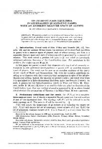
A fuzzy number is a fuzzy set which is defined in R. There are some types of fuzzy numbers [27]. For example, triangular fuzzy numbers (TFNs), trapezoid fuzzy numbers, and etc. We only review TFNs in this paper. The definition of a TFN: A TFN is denoted as (a, b, c), where a ∈ R; b ∈ R; c ∈ R
for short) In the case that (a, b) is a critical point, the first derivatives
Journal of Game Theory 2015, 4(3): 45-55
and ( a ≤ b ≤ c) . The TFN (a, b, c) is described in Figure 1.
47
where
= µ A ( x) {µ A1 ( x1 ), µ A2 ( x1 ),...µ An ( x1 )}, µ A ( x) ∈ ∆ n ( µ A ( x)) ;
1
= µ B ( y ) {µ B1 ( y1 ), µ B2 ( y1 ),...µ Bm ( y1 )}, µ B ( y ) ∈ ∆ m ( µ B ( y )) .
a
b
x
c
Figure 1. Triangular fuzzy number (a, b, c)
The membership function of the TFN (a, b, c) is defined as
x ∈U1 and y ∈U 2 ; n is the number of entries in T1 ( x) ; m is the number of entries in T2 ( y ) ; R = ( rij ) is a n × m matrix, which is called the consequence matrix [22]. It was proved that the fuzzy average converges to arithmetic mean under specific conditions [22]. µ A ( x) is interpreted as the weight of element i
xi ∈ T1 ( x) . For a given x ∈U1 and y ∈U 2 , the vector µ A ( x) , µ B ( y ) is interpreted as probability distribution over T1 ( x) , T2 ( y ) , respectively.
x − a if x ∈ [a, b) b − a c − x = µ ( x) if x ∈ (b, c] In game theory, the set of strategies c − b = S ( = s ,..., s )( i 1, 2,... n ) can be interpreted as the i i1 ik otherwise 0 term set T ( Si ) in the concept of linguistic variables. For There are two special TFNs. One is (a, a, c), such as a = b, example, for a rock-scissors-paper game, a player’s strategy and the other is (a, c, c), such as b = c. Suppose the set S = ( r , s, p ) can be considered as term set of {rock, membership function of TFN (a, a, c), (a, c, c) is µ ( x) , scissors, paper} in linguistic variables, such as ν ( x) , respectively. Then one has the following. T1 ( S ) = {r , s, p} . For two player games in normal form, when player’s 1 c ; (a 0 , then ui ( Pi , P−i ) reaches a local
Theorem 1
=j 1
2
If Di > 0 and Ai < 0 , then, ui ( Pi , P−i ) reaches a
k
∑
a1 x + b1
,...,
µl ( x )
k
µk ( x)
∑
=l 1
,
k
∑
k
∑
µl ( x )
a2 x + b2
k
∑
( al ) x + bl ( al ) x + =l 1 =l= 1 l 1 =l 1 ...,
k
∑
ak x + bk
k
∑
( al ) x + =l 1 =l 1
) bl
)
, bl .
Journal of Game Theory 2015, 4(3): 45-55
P2 ( y ) = (
ν1 ( y )
k
∑
,
ν 2 ( y)
k
∑ ν l ( y)
ν l ( y) =l 1 =l 1
=(
k
c1 y + d1
,
k
∑
∑
k
c2 y + d 2
ν l ( y)
k
∑ ν l ( y)
=l 1
k
∑
,...,
∑
,...,
49
k
)
ck y + d k
k
∑
∑
( cl ) y + dl ( cl ) y + dl ( cl ) y + =l 1 =l = 1 l 1 =l 1 =l 1 =l 1
). dl
Then the derivative of P1 ( x) , P2 ( y ) is the following. k
k
a1 ∑ bl − b1 ∑ al
k
k
k
a2 ∑ bl − b2 ∑ al
k
ak ∑ bl − bk ∑ al
dP1 ( x)=l 1 =l 1 =l 1 =l 1 =l 1 =l 1 =( k , k ,..., k ) k k k dx 2 2 2 ((∑ al ) x + ∑ bl ) ((∑ al ) x + ∑ bl ) ((∑ al ) x + ∑ bl ) =l 1 =l 1 =l 1 =l 1 k
k
c1 ∑ dl − d1 ∑ cl
k
=l 1 =l 1
k
k
c2 ∑ dl − d 2 ∑ cl
k
ck ∑ dl − d k ∑ cl
dP2 ( y= ) =l 1 =l 1 l 1 =l 1 =l 1 = ( kl 1 = , k , ..., k ) k k k dy 2 2 2 ((∑ cl ) y + ∑ dl ) ((∑ cl ) y + ∑ dl ) ((∑ cl ) y + ∑ dl ) =l 1 =l 1 =l 1 =l 1
=l 1 =l 1
It is clear that the elements in each derivative vector have common denominator, the numerator of each element in the above derivative vectors is a constant. On the other hand, the elements in vector Pi (i = 1, 2) have common denominator, and the numerator of each element in vector Pi (i = 1, 2) is a piecewise linear function. Because we can ignore the common denominators in each equation of (3.4), then the first equation in (3.4) finally becomes a linear equation of y, the second equation in (3.4) becomes a linear equation of x. Therefore, equation (3.4) becomes a system of linear equations of x and y. Q.E.D.
4. Examples Three examples are described in this section. Example 1 - Rock- Scissors-Paper game. Find mixed NE for a Rock-Scissors-Paper Game with the following payoff bi-matrix.
rock rock (0, 0) paper (−1,1) scissors (1, −1)
paper (1, −1) (0, 0) (−1,1)
scissors (−1,1) (1, −1) (0, 0)
This is a 2-player symmetric game. The payoff matrices of player 1 and player 2 are as follows.
0 1 − 1 A12 = −1 0 1 , A21= 1 − 1 0 We
build
two
linguistic
values
T
0 − 1 1 1 0 − 1 = A12 . −1 1 0
( Si , Ti ( Si ), U i , Gi , M i )(i = 1, 2) .
= U i [0, = 1](i 1, 2) , and semantic rule M i is defined as follows.
Ti ( Si ) = (rock , scissors, paper ) ,
= M1 : T1 ( S1 ) (rock , scissors, paper ) → ( E1 , E2 , E3 ) = M 2 : T2 ( S2 ) (rock , scissors, paper ) → ( H1 , H 2 , H 3 ) , where Ei , H i (i = 1, 2, 3) is a TFN defined in U1 , U 2 , respectively.
50
Lunshan GAO:
An Efficient Algorithm for Finding Mixed Nash Equilibria in 2-Player Games
E= = = We define E1 = (0, 0,1) , E= 2 3 (0,1,1) , and H 1 H 2 (0, 0,1) , H 3 = (0,1,1) . Then, the sum of membership functions µi ( x) , ν i ( y ) of Ei , H i is as follows. 3
∑ l =1
µl ( x)= x + 1 ,
3
∑ ν l ( y)=
2− y.
l =1
dP1 ( x) 1− x x x −2 1 1 P1 ( x) = ( , , ) , and =( , , ), 2 2 1+ x 1+ x 1+ x dx (1 + x) (1 + x) (1 + x) 2 1 1 1 dP ( y ) −1 −1 2 1− y 1− y y =( , , ). P2 ( y ) = ( , , ) , and P1* = ( , , ) 2 2 2 3 3 3 2− y 2− y 2− y dy (2 − y ) (2 − y ) (2 − y ) 2 One can solve the following system of linear equations.
0 1 − 1 1 − y ∂u1 ( P1 , P−1 ) dP1 ( x) T = • A12 • P2 ( y ) = K1 • (−2, 1, 1) • −1 0 1 • 1 − y = 0 ∂P1 dx 1 − 1 0 y 0 1 − 1 1 − x ∂u2 ( P2 , P−2 )= dP2 ( y ) • A • P ( x)T= K • (−1, − 1, 2) • −1 0 1 • x = 0 21 1 2 ∂P2 dy 1 − 1 0 x where K1 =
1 (1 + x) 2 (2 − y )
The solution is x=
1 1 1 P2* = ( , , ) . 3 3 3
and K 2 =
1 (2 − y ) 2 (1 + x)
.
1 1 ∈ [0,1] . The mixed NE ( P1* , P2* ) with probability distributions and ∈ [0,1] , y= 2 2
Let us examine the solution ( P1* , P2* ) for player 1 by using Hessian matrix or step 5 described in the algorithm.
= A1
∂ 2 u1 ( P1 , P2 ) ∂P12
∂ 2 u1 ( P1 , P2 ) B= 1 ∂P1∂P2
P1 = P1*
= *
P2 = P2
d 2 P1 ( x) dx 2
x=
• A12 • P2 ( y )T
dP1 ( x) = • A12 * P2 = P2 dx P1 = P1*
1
2 0, = 1
y= T
dP ( y ) • 2 dy
2 1 2 = 1 y= 2
16 . 9
1 2 = 1 y= 2
0
x=
D1 = A1C1 − B12 < 0 . Therefore, point ( P1* , P2* ) is a saddle point of u1 ( P1 , P2 ) . Let us examine the solution ( P1* , P2* ) for player 2.
A2 =
∂ 2 u2 ( P2 , P1 ) ∂P2 2
∂2u (P , P ) B2 = 2 2 1 ∂P1∂P2
P1 = P1*
=
P2 = P2*
d 2 P2 ( y ) dy 2
x=
T
x=
• A21 • ( P1 ( x) )
dP2 ( y ) dP ( x) • A21 • 1 * = P2 = P2 dy dx P1 = P1*
D2 = A2 C2 − B2 2 < 0 . Thus, point ( P1* , P2* ) is a saddle point of u2 ( P2 , P1 ) . Example 2 - Find mixed NE in the following 2-player game. Player ΙΙ
T
1 2 1 y= 2
16 = − . 9
Journal of Game Theory 2015, 4(3): 45-55
s21
s2 2
51
s23
s11 (1, 1) (3, 1) (2, 2) s12 (2, 4) (2, 5) (8, 3) s13 (3, 3) (0, 4) (0, 1)
Player Ι
1 4 3 1 3 2 A12 = 2 2 8 , A21 = 1 5 4 2 3 1 3 0 0 We define two linguistic values ( S , T ( Si ), U i , Gi , M i )(i ∈ 2) , where U i = [0, 1] , T ( Si ) = {si1 , si 2 , si 3 } (i=1, 2). The semantic rules M i (i=1, 2) are defined as follows.
M1 : T ( S1 ) → {E1 , E2 , E3 } , M 2 : T ( S2 ) → {H1 , H 2 , H 3 } where TFNs Ei , H i (i = 1, 2, 3)
H 3 = (0,1,1) . Then, we have
3
= = E= are defined as follows, E1 = (0, 0,1) , E= 1 H 2 (0, 0,1) , 2 3 (0,1,1) ; H
∑ µi ( x ) =
1 + x and
i =1
3
∑ν i ( y)=
2− y.
i =1
The probability distribution Pi over U i (i=1, 2) is as follows.
µ ( x) µ1 ( x) µ ( x) x 1− x x = P1 ( x) (= , 3 2 , 3 3 ) ( , , ), 3 1+ x 1+ x 1+ x ∑ µi ( x ) ∑ µi ( x ) ∑ µi ( x ) =i 1 =i 1 =i 1
ν 3 ( y) ν1 ( y ) ν 2 ( y) y 1− y 1− y = P2 ( y ) (= , , ) ( , , ) 3 3 3 2− y 2− y 2− y ∑ν i ( y) ∑ν i ( y) ∑ν i ( y) =i 1 =i 1 =i 1
Then, we have
dP1 ( x) dP2 ( y ) −2 1 1 2 −1 −1 =( , , ), , , ) =( 2 2 2 2 2 dx dy (1 + x) (1 + x) (1 + x) (2 − y ) (2 − y ) (2 − y ) 2 One can solve the following system of linear equations.
1 3 2 1 − y ∂u1 ( P1 , P−1 ) = K1 • (−2, 1, 1) • 2 2 8 • 1 − y = 0 ∂P1 3 0 0 y 1 4 3 1 − x ∂u2 ( P2 , P−2 )= K • (−1, − 1, 2) • 1 5 4 • x = 0 2 ∂P2 2 3 1 x where K1 =
1 2
(1 + x) (1 + y )
and K 2 =
1 (1 + y ) 2 (1 + x)
.
52
Lunshan GAO:
An Efficient Algorithm for Finding Mixed Nash Equilibria in 2-Player Games
1 1 ∈ [0, 1] , y= ∈ [0, 1] . This 2-player game has a mixed NE ( P1* , P2* ) with probability 5 5 2 1 1 4 4 1 distribution P1* = ( , , ) and P2* = ( , , ) . 3 6 6 9 9 9 The solution is x=
Let us examine this solution for player 1.
= A1
∂ 2 u1 ( P1 , P2 )
P1 = P1*
=
P2 = P2*
∂P12
∂2u (P , P ) B1 = 1 1 2 ∂P1∂P2
d 2 P1 ( x) dx 2
1 5 = 1 y= 5
x=
T
• A12 • P2 ( y )
dP1 ( x) • A12 * = P2 = P2 dx P1 = P1*
0
1 5 1 y= 5
T
dP ( y ) • 2 dy
x=
4375 = − 2916
D1 = A1C1 − B12 < 0 . Therefore, point ( P1* , P2* ) is a saddle point of u1 ( P1 , P2 ) . Let us examine the solution for player 2.
= A2
∂ 2 u2 ( P2 , P1 )
P1 = P1*
= *
∂P2 2
P2 = P2
∂2u (P , P ) B2 = 2 2 1 ∂P1∂P2
d 2 P2 ( x) dy 2
x=
• A21 • P1 ( y )T
y= T
dP2 ( y ) dP ( x) • A21 • 1 * = P2 = P2 dy dx P1 = P1*
1
5 0 = 1 5 1 5 1 y= 5
x=
1250 = − 486
D2 = A2 C2 − B2 2 < 0 . Thus, point ( P1* , P2* ) is a saddle point of u2 ( P2 , P1 ) . Example 3 - Find mixed NE for the following bi-matrix game. Player ΙΙ
a1 s1 s2 s3 s4 s5
Player Ι
0 −1 1 A12 = 1 1
( 0, 0) (-1, 1) ( 1, 0) ( 1,-1) ( 1, -1)
1
1
0 −1 −1 0
1 0 1 −1
a2
a3
( 1,-1)
( 1, 1)
a4
(-1, 0) ( 0, 1) ( 1, 0) ( 0, 0) (-1,-1) ( 0, 1) (-1, 1) (-1, 0) ( 1,-1) ( 0, 0) ( 0, 0) (-1,-1) ( 0, 0)
−1 0 0 −1 − 1 , A21 = 1 0 0 0
1 1 0 0
0
−1
− 1 −1 0 0 1 −1 −1 1 0 0
We build two linguistic values ( Si , Ti ( Si ), U i , Gi , M i )(i ∈ 2) . T1 ( S1 ) = ( s1 , s2 , s3 , s4 , s5 ) on U1 = [0, 1] . T2 ( S2 ) = (a1 , a2 , a3 , a4 ) on U 2 = [0, 1] , and the semantic rule M i is defined as follows.
= M1 : T1 ( S1 ) ( s1 , s2 , s3 , s4 , s5 ) → ( E1 , E2 , E3 , E4 , E5 ) = M 2 : T2 ( S2 ) (a1 , a2 , a3 , a4 ) → ( H1 , H 2 , H 3 , H 4 ) where Ei (i = 1, 2, 3, 4, 5) and H i (i = 1, 2, 3, 4) are TFNs defined in U1 and U 2 as follows.
Journal of Game Theory 2015, 4(3): 45-55
5
E= E= E= 1 E= 2 (0, 0,1) , E= 3 4 5 (0,1,1)
∑ µi ( x)=
2 + x and
i =1
4
∑ν i ( y)= i =1
and
53
H1 = (00,1) , H= H= H= 2 3 4 (0,1,1) . Then, we have
1 + 2 y . The probability distribution Pi over U i (i=1, 2) is as follows.
µ ( x) µ ( x) µ1 ( x) µ ( x) µ ( x) 1− x 1− x x x x P1 ( x) (= , 5 2 , 5 3 , 5 4 , 5 5 ) ( , , , , ), 5 2+ x 2+ x 2+ x 2+ x 2+ x ∑ µi ( x ) ∑ µi ( x ) ∑ µi ( x ) ∑ µi ( x ) ∑ µi ( x ) =i 1 =i 1 =i 1 =i 1 =i 1
ν ( y) ν1 ( y ) ν ( y) ν ( y) 1− y y y y P2 ( y ) (= , 42 , 43 , 44 ) ( , , , ) 4 1+ 2y 1+ 2y 1+ 2y 1+ 2y ∑ν i ( y) ∑ν i ( y) ∑ν i ( y) ∑ν i ( y) =i 1 =i 1 =i 1 =i 1
Then, we have
dP1 ( x) −3 −3 2 2 2 =( , , , , ), 2 2 2 2 dx (2 + x) (2 + x) (2 + x) (2 + x) (2 + x)2 dP2 ( y ) −3 1 1 1 =( , , , ). 2 2 2 dy (1 + 2 y ) (1 + 2 y ) (1 + 2 y ) (1 + 2 y ) 2 One can solve the following system of linear equations.
0 1 1 −1 1 − y ∂u ( P , P ) −1 0 1 0 y = 0 1 1 2 = K1 • (−3, − 3, 2, 2, 2) • 1 − 1 0 − 1 • ∂P1 y 1 − 1 1 0 y 1 0 − 1 0 1 − x 0 1 0 1 1 − − 1 − x ∂u2 ( P2 , P−2 ) −1 1 − 1 0 0 = K 2 • (−3, 1, 1 1) • • x = 0 1 0 1 1 1 − − P ∂ 2 x 0 0 1 0 0 x where K1 =
1 2
(2 + x) (1 + 2 y )
and K 2 =
1 (1 + 2 y ) 2 (2 + x)
.
2 3 ∈ [0, 1] , y= ∈ [0, 1] . This 2-player game has a mixed NE ( P1* , P2* ) with probability 7 7 4 3 3 3 5 5 2 2 2 distribution P1* = ( , , , , ) and P2* = ( , , , ) . 13 13 13 13 16 16 16 16 16 The solution is x=
Let us examine this solution ( P1* , P2* ) for player 1. 2
x= d 2 P1 ( x) ∂ 2 u1 ( P1 , P2 ) P1 = P1* T 7 0 A1 = A P ( y ) = = 12 2 * 3 P2 = P2 y= dx 2 ∂P12 7
∂ 2 u1 ( P1 , P2 ) B1 = ∂P1∂P2
T
dP1 ( x) dP ( y ) A12 2 * = P2 = P2 dx dy P1 = P1*
D1 = A1C1 − B12 < 0 . Thus, point ( P1* , P2* ) is a saddle point of u1 ( P1 , P2 ) .
2 7 3 y= 7
x=
= −
93639 . 43264
54
Lunshan GAO:
An Efficient Algorithm for Finding Mixed Nash Equilibria in 2-Player Games
Let us examine this solution ( P1* , P2* ) for player 2.
= A2
∂ 2 u2 ( P2 , P1 ) ∂P2 2
∂ 2 u2 ( P2 , P1 ) B= 2 ∂P1∂P2
P1 = P1*
=
P2 = P2*
d 2 P2 ( y ) dy 2
2 7 = 3 y= 7
x=
T
• A21 • P1 ( x)
T
dP2 ( y ) dP ( x) = • A21 • 1 * P2 = P2 dy dx
P1 = P1*
0
2 7 = 3 y= 7
x=
2401 2704
D2 = A2 C2 − B2 2 < 0 . Therefore, point ( P1* , P2* ) is a saddle point of u2 ( P2 , P1 ) .
5. Conclusions This paper shows that computing mixed NE in bi-matrix games is equivalent to solving a system of linear equations. It is proved that the new algorithm can calculate mixed NE in 2-player games within polynomial time. We claim that there is a fully polynomial time scheme of calculating mixed NE in 2-player games. The algorithm can also be applied to multiplayer games if a multiplayer game is able to be reduced to a group of 2-player games. Future study will conduct to compare the new algorithm with exiting algorithms, and to apply the new algorithm to dynamic game theory and evolutionary game theory.
ACKNOWLEDGMENTS The author would like to thank anonymous reviewers’ comments and suggestions.
REFERENCES
Vol. 56, Issue 3, 2009. [9]
X. Chen, D. Durfee, and A. Orfanou, "On the Complexity of Nash Equilibria in Anonymous Games", at arXiv: 1412.5681vl, Dec. 2014.
[10] X. Chen, D. Paparas, and M. Yannakakis, "The complexity of non-monotone markets", In Proceeding of the 45th Annual ACM Symposium on Theory of Computing, pp.181-190, 2013. [11] S. Cheng, D. Reeves, Y. Vorobeychik and M. Wellman, "Notes on Equilibria in Symmetric Games", In the Proceeding of the 6th International workshop on Game-Theoretic and Decision-Theoretic Agents, 2004. [12] L. Cigler and B. Faltings, "Symmetric Subgame-Perfect Equilibria in Resource Allocation", Journal of Artificial Intelligence Research 49, pp.323-361, 2014. [13] C. Daskalakis, "An efficient PTAS for two-strategy anonymous games", In Proceedings of the 4th International Workshop on Internet and Network economics, pp.186-197, 2008. [14] C. Daskalakis, P. W. Goldberg, C. H. Papadimitriou, “The Complexity of Computing a Nash Equilibrium”, ECCC, TR05-115, 2005.
[1]
T. Basar and G. J. Olsder, "Dynamic Noncooperative Game Theory", 2nd edition, SIAM, 1995.
[15] C. Daskalakis, and C. H. Papadimitriou, “Three-Player Games are Hard”, ECCC, TR05-139, 2005.
[2]
Bellman R. E. and L. A. Zadeh, Decision making in a fuzzy environment, Management science, 17(1970), pp.141-164.
[3]
V. D. Blondel and J. N. Tsitsiklis, "A Survey of Computational Complexity Results", Automatica 36 (2000), pp. 1249-1274, Elsevier.
[16] C. Daskalakis and C. H. Papadimitriou, "Computing equilibria in anonymous games", In Proceedings of the 48th Annual IEEE Symposium on Foundations of Computer Science, pp.83-93, 2007. [17] C. Daskalakis and C. H. Papadimitriou, "Discretized multinomial distributions and Nash equilibira in anonymous games" In Proceedings of the 49th Annual IEEE Symposium on Foundations of Computer Science, pp.25-34, 2008.
[4]
F. Brandt, F. Fischer and M. Holzer, "Symmetries and Complexity of Pure Nash Equilibrium", Journal of Computer and System Sciences, 2009 Elsevier.
[5]
D. Butnariu, "Fuzzy Games: A Description of Time Concept", Fuzzy Sets and Systems, Vol. 1, pp. 181–192, 1978.
[18] C. Daskalakis and C. H. Papadimitriou, "On oblivious PTAS's for Nash equilibrium", In Proceedings of the 4th Annual ACM Symposium on Theory of Computing, pp.75-84, 2009.
[6]
A. Chakeri and F. Sheikholeslam, "Fuzzy Nash Equilibriums in Crisp and Fuzzy Games", IEEE Transactions on Fuzzy Systems, 2012 IEEE.
[19] L. Gao, “Finding Nash Equilibria for Polymatrix Games”, International Journal of Computer Science and Artificial Intelligence”, Vol. 5, Iss. 1, pp. 1-10, 2015.
[7]
X. Chen and X. Deng, “3-Nash is PPAD-complete”, ECCC, TR05-134, 2005.
[8]
X. Chen, X. Deng and S. Teng, “Settling the Complexity of Computing two-player Nash Equilibria”, Journal of the ACM,
[20] L. Gao, “A Direct Algorithm for Computing Nash Equilibriums”, International Journal of Computer Science and Artificial Intelligence, Vol. 3, Iss. 2, pp. 80-86, 2013. [21] L. Gao, “The Discussion of Applications of the Fuzzy
Journal of Game Theory 2015, 4(3): 45-55
Average to Matrix Game Theory”, The Proceeding of CCECE2012, May 2012. [22] L. Gao, “The Fuzzy Arithmetic Mean”, Fuzzy Sets and Systems, 107, No. 3 pp. 335-348, 1999. [23] D. Garagic and J. B. Cruz, Jr, "An Approach to Fuzzy Noncooperative Nash Games", Journal of Optimization Theory and Applications. Vol. 118, No.3, pp. 475-491, 2003.
55
Mathematics, Vol. 54, Iss. 2 pp286-295, 1951. [30] Von Neumann, Morgenstern, Theory of Games and Economic Behavior, Princeton University Press, 1944. [31] R. Porter, E. Nudelman and Y. Shohem, “Simple Search Methods for Finding a Nash Equilibrium”, Games and Economic Behavior 63 (2008), pp642-662 Elsevier.
[24] P. W. Goldberg and A. Turchetta, "Query Complexity of Approximate Equilibria in Anonymous Games", arXiv: 1412.6455v2, Apr. 2015.
[32] C. T. Ryan, A. Jiang and K. L. Brown, "Computing Pure Strategy Nash Equilibria in Compact Symmetric Games", The Proceeding of 11th ACM Conference on EC, June 7-11, 2010.
[25] A. M. Hefti, "Uniqueness and Stability in Symmetric Games: Theory and Applications", ECON working paper, 2013.
[33] W. H. Sandholm, “Lecture Notes on Game Theory”, 2014, at www.ssc.wisc.edu/~whs/teaching/711/lngt.pdf.
[26] J. Horner, N. Klein, and S. Rady, "Strongly Symmetric Equilibria in Brandit Games", 2013 https://www.economicd ynamics.org/meetpapers/2013/paper_1107.pdf.s.
[34] W. H. Sandholm, "Evolutionary Game Theory", at www.ssc.wisc.edu/~whs/research/edt.pdf.
[27] A. Kaufmann, and M. M. Gupta, Fuzzy Mathematical Models in Engineering and Management Science, Elsevier, Amsterdam, 1998. [28] R. Mehta, V. V. Vazirani and S. Yazdanbod, “On Settling Some Open Problems on 2-Player Symmetric Nash Equilibria”, The Proceeding of 8th International Symposium on Algorithmic Game Theory, SAGT2015. [29] J. Nash, "Non-Cooperative Games", The Annals of
[35] S. H. Wu, and V. W. Soo, "A Fuzzy Theoretic Approach to Multi-Agent Coordination, Multiagent Platforms, Springer Verlag, New York, NY, pp. 76–87, 1998. [36] L. A. Zadeh, “The Concept of Linguistic Variable and its Application to Approximate Reasoning-1”, Information Sciences, 8, pp.199-249, 1975. [37] H. J. Zimmermann, Fuzzy Set Theory and Its Application, 2nd edition, Kluwer Academic Publishers, Boston, 1991.