Working Paper No. 2010/58 Fiscal Decentralization and Urbanization in Indonesia Margherita Comola1 and Luiz de Mello2 May 2010 Abstract Indonesia went through a process of fiscal decentralization in 2001 involving the devolution of several policymaking and service delivery functions to the subnational tiers of government (provinces and districts). This process is likely to have affected regional patterns of urbanization, because the new prerogatives granted to the local governments have altered the distribution of urban amenities and labour market outcomes among and within the local jurisdictions. This paper uses a dataset of local governments for 1996 and 2004-05 to estimate the effect of the decentralization of minimum-wage setting in 2001 on urban population growth. Our findings suggest that, controlling for demand- and supply-side determinants of urban population growth, if the minimum wage had risen by an additional 81.5 thousand rupiah (25 per cent of its initial mean value), the urban population would have risen by an additional 0.4 per cent from its initial level. Keywords: Indonesia, minimum wage, federalism, urbanization JEL classification: H72, J61, R23
Copyright © UNU-WIDER 2010 1 Paris
School of Economics, Paris, email:
[email protected]; 2 OECD Economics Department, Paris Cedex 16, email:
[email protected]; This study has been prepared within the UNU-WIDER project Asian Development in an Urban World, directed by Jo Beall, Basudeb Guha-Khasnobis and Ravi Kanbur. UNU-WIDER acknowledges the financial contribution to its research programme by the governments of Denmark (Royal Ministry of Foreign Affairs), Finland (Ministry for Foreign Affairs), Sweden (Swedish International Development Cooperation Agency—Sida) and the United Kingdom (Department for International Development). ISSN 1798-7237
ISBN 978-92-9230-295-5
Acronyms DAK earmarked or conditional transfers (dana alokasi khusus) DAU general allocation grant (dana alokasi umum) SDA sharing of oil and gas revenue
The World Institute for Development Economics Research (WIDER) was established by the United Nations University (UNU) as its first research and training centre and started work in Helsinki, Finland in 1985. The Institute undertakes applied research and policy analysis on structural changes affecting the developing and transitional economies, provides a forum for the advocacy of policies leading to robust, equitable and environmentally sustainable growth, and promotes capacity strengthening and training in the field of economic and social policy making. Work is carried out by staff researchers and visiting scholars in Helsinki and through networks of collaborating scholars and institutions around the world. www.wider.unu.edu
[email protected]
UNU World Institute for Development Economics Research (UNU-WIDER) Katajanokanlaituri 6 B, 00160 Helsinki, Finland Typescript prepared by Liisa Roponen at UNU-WIDER The views expressed in this publication are those of the author(s). Publication does not imply endorsement by the Institute or the United Nations University, nor by the programme/project sponsors, of any of the views expressed.
1
Introduction
Indonesia went through an ambitious process of fiscal and administrative decentralization in 2001, according to which several political, policymaking and service delivery functions were transferred to the lower tiers of government. Of particular interest was the devolution of minimum-wage setting to the local governments and provinces. This process is likely to have affected regional patterns of urbanization, because the new prerogatives granted to the local governments, coupled with growing political autonomy, have altered the distribution of infrastructure (urban amenities) and labour market outcomes among and within the local governments. At about 50 per cent, Indonesia’s urbanization rate is in line with the average of low-income countries, but there is considerable regional variation within the country in urbanization rates and trends. Against this background, this paper describes trends in urbanization across the Indonesian local jurisdictions and discusses how a particular feature of decentralization —minimum-wage setting—is likely to have affected urban population growth and the distribution of the local population between cities and rural areas. Theoretical motivation is derived from two strands of literature. One is based on the conventional models of urbanization, following the tradition of Brueckner (1990), according to which urban population growth is driven primarily by differences in income and market potential between urban and rural areas. The other is inspired by De Long and Shleifer (1993), Ades and Glaeser (1995), Davis and Henderson (2003) and Henderson and Wang (2007) and considers the effects of institutions, including federalism and democratization, on urbanization and urban concentration. Previous research on the effects of fiscal decentralization on urbanization and regional development includes Firman (2003). Empirical evidence is provided for a dataset of Indonesian local governments constructed primarily on the basis of the labour market (Sakernas), household (Susenas) and industrial (Survei Industri) surveys. Using the local governments as the units of observation, we estimate the effect of decentralization of minimum-wage setting in 2001 on urban and rural population growth in a reduced-form setting that controls for the supply and demand drivers of urbanization. We focus on changes in the relevant variables between 1996 and 2004-05,1 a time span that covers the pre- and postdecentralization periods. We differ from previous empirical literature in two main ways: we focus on a cross-section of local governments within a single country, rather than on a cross-section of countries, and use household and labour market survey, rather than population census, data. Our main finding is that, controlling for demand and supply factors, an increase in the minimum wage is associated with an increment in the urban population at the district level. In particular, controlling for other determinants of urban population growth, if the minimum wage had risen by 81.5 thousand rupiah (25 per cent of its initial mean value), the urban population would have risen by an additional 0.4 per cent from its initial level.
1 While Sakernas is carried out every year, the consumption/expenditure module of Susenas is available every four years. Thus, Sakernas data refer to 2004 and Susenas data to 2005.
1
The paper is organized as follows. Section 2 overviews the main features of urbanization in Indonesia. Section 3 describes the estimation procedure and the dataset. Section 4 presents the estimation results, and Section 5 concludes.
2
Minimum wage, decentralization and urbanization
2.1 Urbanization in Indonesia Indonesia’s urban population nearly has doubled since 1990 to about 109 million in 2005, the latest year for which mid-census data are available. The country’s urbanization rate is in the neighbourhood of 50 per cent, which is in line with the average of low-income countries, and is estimated to rise to nearly 69 per cent in 2030 (United Nations 2007). As in other developing countries, rural/urban migration has been the main engine of city growth in Indonesia. The urban population grew by over 4.5 per cent per year on average during 1985-05, while the rural population shrank by 0.3 per cent per year on average over the same period. Net migration is estimated to have accounted for almost 60 per cent of urban growth in Indonesia in the 1980s (United Nations 2001). Nevertheless, Indonesia’s rural population, although declining, is among the largest in the world, at about 117 million in 2005. This suggests ample room for further rural emigration to continue to sustain rapid urbanization. Of course, population census-based urbanization trends, although illustrative, need to be assessed with some caution. For example, they are affected by changes in the classification of localities between urban and rural, which is often based on administrative criteria that not always reflect differences in economic structure between urban and rural areas (Hugo 2003; Firman, Kombaitan and Pradono 2007).2 We go some way in addressing this problem by using household and labour market survey data. To illustrate these methodological differences, basic urbanization indicators are reported in Table 1 for 1996 and 2004, the reference years used in the empirical analysis below. Table 1 Urbanization indicators, 1996 and 20040-05, % Population censusa
Sakernas
1996 2004 Note:
Urban
Rural
Urban
Rural
42.9 49.9
57.1 51.0
35.6 48.1
64.4 51.9
a refers to 1995 and 2005 (mid-census years), instead of 1996 and 2004.
Source: Susenas, Sakernas, and United Nations (2007).
2 This is important, because the distinction between urban and rural areas has become increasingly blurred, reflecting to a large extent an increasingly complex mix of activities in urban and peri-urban areas and along transport corridors connecting large urban centres. In the case of Indonesia, for example, this phenomenon is often referred to as kotadesasi (McGee 1991, 1992; Firman 1992; Firman, Kombaitan and Pradono 2007).
2
There is a limited empirical literature on the determinants of urbanization in Indonesia. Firman Kombaitan and Pradono (2007) discuss the main determinants of urbanization since the 1980s and attribute the concentration of population and economic activity in the Jakarta Metropolitan Area (Jabotabek) to the country’s integration into the world economy. Firman (1992) uses census data to describe the patterns of urban population growth in 82 Javanese predominantly rural districts (kapubaten) during 1980-90, excluding Jakarta and the districts that are predominantly urban (kota). Consistent with our approach, the unit of observation is the local governments (kabupaten/kota). The author reports a trend towards comparatively higher urban population growth in the large cities and in their surrounding areas. When discussing the main determinants of urban concentration in the metropolitan areas of Jakarta and Bandung, Firman (2003 and 2009) relates urbanization and fiscal decentralization through the empowerment of local governments, which is expected to better tailor the provision of urban amenities and infrastructure to local needs. 2.2 An overview of Indonesia’s decentralization process Following the demise of the Suharto regime in 1998, Indonesia launched an ambitious fiscal decentralization programme that was implemented from 2001. Decentralization allowed for increasing demands for policymaking autonomy at the subnational level to be met in a country that is characterized by considerable economic and geographic diversity. ‘Big-bang’ decentralization was implemented smoothly, despite serious administrative and capacity constraints at the local level and without serious disruption in service delivery. Fiscal and administrative decentralization was taken a step further in 2004, when direct elections (Pilkada Langsung) were introduced for province governors and heads of local governments. Decentralization has put the local, rather than the middle-tier, jurisdictions at the forefront of service delivery. Several expenditure assignments, especially in the social area, were decentralized to the local governments, which now account for almost two-thirds of consolidated government spending, nearly double the pre-decentralization share. Notwithstanding their increased expenditure assignments, the local governments have limited taxing autonomy: income and property tax revenue is collected by the centre and transferred to the local governments on a derivation basis. The bulk of local government revenue comes from a general allocation grant (DAU, dana alokasi umum), followed by the sharing of oil and gas revenue (SDA) and earmarked or conditional transfers (DAK, dana alokasi khusus), which are used to finance predominantly capital outlays. Own sources account for less than 10 per cent of local government revenue. DAU is financed through a fixed share of central government net revenue (currently 26 per cent), of which 90 per cent is allocated to the local governments and the remainder is allocated to the provinces. In addition to increasing vertical imbalances, decentralization has exacerbated horizontal inequality among the local governments. This is essentially because the sharing of revenue from the exploitation of natural resources is limited to the oil- and gas-rich provinces. Also, there is limited scope for using DAU as an equalization tool, because funds are distributed among the local governments on a derivation basis, rather than in relation to estimated fiscal capacity and expenditure needs. Another consideration is that, although DAU allocations are intended to be formula-based, they are still guided in part by historical budgeting on the basis of pre-decentralization
3
appropriations for the formerly deconcentrated personnel and assets that have subsequently been decentralized to the regional governments (Hofman et al. 2006). At the same time, the central government retains control over the regional governments in areas related to tax policy (by setting tax bases and ranges for rates), budget making (local budgets need to be submitted to and approved by the central government), financial management (there are constraints on local government borrowing and debt management) and investment programmes, including in devolved sectors, such as education, health care and infrastructure development. Following decentralization, there was a proliferation of subnational jurisdictions. The number of local governments (both kapubaten and kota) rose from 314 in 1998 to 440 at end-2005, and five provinces were created over this period, raising their number to 33. Legal constraints on the creation of new jurisdictions are lax and incentives for fragmentation are strong, given the reliance of local governments on financing from the centre, as well as bureaucratic and political rentseeking in some cases (Fitrani, Hofman and Kaiser 2005). Of particular importance for our empirical analysis is the devolution of minimum-wage setting to the subnational governments in 2001.3 The minimum wage is currently calculated by the local governments on the basis of an estimated cost-of-living indicator and then proposed to the provincial governments by a tri-partite wage council, including representatives from labour, government and the private sector. Typically, the provinces set the minimum wage at the level proposed by the local governments.4 By contrast, prior to decentralization, the minimum wage used to be set nationally by the central government on the basis of a different cost-of-living indicator. Following decentralization, the minimum wage rose considerably in real terms, especially during 2000-03, reaching about 65 per cent of the median wage in 2004, a ratio that is far higher than the 45 per cent average of the OECD area (OECD 2008; Comola and de Mello 2009, 2010). 2.3 How may decentralization affect urbanization? There are several channels through which the devolution of service delivery and minimum-wage setting to sub-national governments, coupled with greater political autonomy, may affect the supply-demand mix for urbanization. First, decentralization has granted the local jurisdictions increasing autonomy to allocate their budgetary resources among competing needs. This is despite the fact that several expenditure functions are still costed on the basis of historical budget allocations and financed through transfers from the centre. Moreover, there is considerable anecdotal evidence that capacity constraints in the areas of budget making and expenditure management have had a bearing on the ability of local governments to implement
3 For more information on minimum-wage setting, see SMERU (2001) and Widartu (2006). See also Comola and de Mello (2010) for empirical evidence on the effect of the minimum wage on employment and earnings using a multinomial selection model. 4 Until end-2000, there were different minimum wages within a few provinces (Riau, South Sumatra, West Java, East Java and Bali) and for selected sectors of activity.
4
Table 2 Infrastructure indicators: Urban and rural areas, 1996 and 2005 Access rates, in % of households 1996 Sources of drinking water Piped water Pump Well Spring Other Toilet facilities Private Shared Other
2005
rural
urban
rural
urban
43.9 16.5 34.1 2.4 3.2
7.6 6.7 50.8 20.8 14.1
6.4 37.0 44.6 7.7 4.4
1.0 9.8 40.8 27.8 20.6
65.7 16.0 18.3
39.8 11.0 49.2
72.7 15.0 12.3
50.8 11.1 38.1
Source: Susenas.
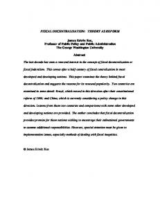
infrastructure development projects. Notwithstanding these caveats, urban-rural infrastructure differentials have shrank somewhat over time, although there is no clear pattern across indicators (Table 2). Second, by devolving minimum-wage setting to the districts and provinces, decentralization may have resulted in greater wage dispersion across the regions. This is important for our empirical analysis. Until 2000, there appears to have been a process of gradual reduction in disparities in the value of the minimum wage across jurisdictions, with higher real increases in the local governments and provinces where the minimum wage had the lowest values (Comola and de Mello 2009). However, decentralization seems to have put a halt to this process of minimum-wage convergence (Figure 1). As wage is a key determinant of rural-urban migration (both within and across districts), the decentralization of minimum-wage setting is likely to have played a role in the process of urbanization and to have affected some local governments more than others. An important consideration is that minimum-wage provisions apply only to full-time regular workers and are not enforced among informal sector workers. This is interesting for empirical hypothesis testing, because it can be used as an identification device: changes in the minimum wage can be used to identify an effect of decentralization that is circumscribed to urban areas. Of course, there are informal sector workers in urban areas, but it can be assumed that rural employment is essentially informal. Labourmarket survey (Sakernas) data indeed suggest that over 91 per cent of employment in rural areas was informal in 2004, against about 56 per cent in the urban areas (Comola and de Mello 2009).5
5 To some extent, earnings in the informal sector are affected by wage-setting in the formal sector, but this hypothesis cannot be tested in Indonesia, because the labour-market survey does not report information on earnings for informal-sector workers. See Comola and de Mello (2010) for more information.
5
Figure 1 Minimum-wage setting and decentralization, 1988-2006 A. Before decentralisation
1
Real change in minimum wage during 1988-2000 (%) 60 45 30
y = -0.9408x + 48.489 R² = 0.5313
15 0 -15 -30 15
25
35
45
55
65
75
85
Minimum wage in 1988 (in thousands of rupiah) B. After decentralisation
1
Real change in minimum wage during 2001-06 (%) 25 20 y = -0.0396x + 20.049 R² = 0.1734
15 10 5 0 -5 200
250
300
350
400
450
Minimum wage in 2001 (in thousands of rupiah)
Note: 1. The diamonds refer to the minimum wage at the provincial level. Average yearly changes are deflated by the GDP deflator. Source: Ministry of Manpower and World Bank (WDI).
3
The estimating strategy
3.1 The theoretical hypothesis There is widespread agreement that the demand for urbanization is driven primarily by differences in income and the stock of amenities (adjusted for cost-of-living differentials) between cities and rural areas.6 Individuals decide to move to the city in
6 See Brueckner (1990), for example, for a review of the early literature on developing countries; Glaeser, Scheinkman and Shleifer (1995) and Black and Henderson (2003) for a more general
6
search of better job opportunities, and because they believe the quality of life to be better than in rural areas. Accordingly, the demand for urbanization can be defined as:
⎛ U y Uj U AUj U ⎞ ⎜ U = U yi , ∑ j , j ≠i , Ai , ∑ j , j ≠i , Pi ⎟ , ⎜ ⎟ τ τ ij ij ⎝ ⎠ d i
d i
(1)
where y ik denotes per capita income in jurisdiction i (among the existing N jurisdictions) for place of residence k, which can be urban (U) or rural (R); Aik is the stock of amenities in jurisdiction i for place of residence k; τ ij is the average distance between jurisdictions i and j; and PiU is the urban population in jurisdiction i, used as a scale variable. The supply of residents from outside the city also depends on income differentials, the stock of amenities in rural areas in the reference jurisdiction and in neighbouring jurisdictions (adjusted for distance), and the size of the rural population in the reference district. As a result, the supply of migrants to the city can be defined as:
⎛ y Rj A Rj R ⎞ U is = U is ⎜ yiR , ∑ j , j ≠i , AiR , ∑ j , j ≠i , Pi ⎟ ⎜ ⎟ τ τ ij ij ⎝ ⎠,
(2)
where Pi R is the rural population in jurisdiction i. In equilibrium, where U id = U is = U i , the size of the urban population in the reference jurisdiction can be computed by solving Equations (1) and (2) for PiU , such that:
⎛ yUj y Rj AUj A Rj ⎞ ⎟. , ∑ j , j ≠i , AiU , AiR , ∑ j , j ≠i , ∑ j , j ≠i PiU = PiU ⎜ Pi R , yiU , yiR , ∑ j , j ≠i ⎜ ⎟ τ τ τ τ ij ij ij ij ⎝ ⎠
(3)
We argue that decentralization affects indirectly the demand and supply determinants of urbanization through its impact on income through minimum-wage setting. Because of non-enforcement of minimum-wage provisions in the rural sector, as discussed above, we make the identifying assumption that y iU = y iU ( MWi ) , where MWi is the minimum wage in the reference jurisdiction. As a result, Equation (3) can be re-written as:
⎛ yUj y Rj AUj A Rj ⎞ R R U R ⎟. Pi = Pi ⎜ MWi , Pi , yi , Ai , Ai , ∑ j , j ≠i , ∑ j , j ≠i , ∑ j , j ≠i , ∑ j , j ≠i ⎜ ⎟ τ τ τ τ ij ij ij ij ⎝ ⎠ U
U
(4)
Equation (4) can be estimated for first-differenced data using the 1996 (before decentralization) and 2004/2005 (after decentralization) waves of the survey data used to construct our dataset (described below), such that:
theoretical model and evidence on the determinants of city growth; and Duranton and Puga (2004) for a theoretical model.
7
⎛ y Uj y Rj AUj A Rj ⎞ R R U R ⎜ ⎟ . (5) ΔPi = ΔPi ΔMWi , ΔPi , Δyi , ΔAi , ΔAi , ∑ j , j ≠i , ∑ j , j ≠i , ∑ j , j ≠i , ∑ j , j ≠i ⎜ ⎟ τ τ τ τ ij ij ij ij ⎠ ⎝ U
U
3.2 Estimating equation
Equation (5) is a reduced-form equation relating changes in the size of the urban population to changes in the minimum wage. However, its estimation poses a few initial methodological challenges. First, population growth is known to be persistent (Rappaport 2004), which affects the error structure of the estimating equation. We deal with this problem by including the initial value of the urban and rural populations among the regressors. Second, ΔPi R and Δy iR , as well as changes in the amenity indicators, are most likely endogenous, which would bias the parameter estimates. Estimation by IV is difficult, because it would raise the issue of the appropriateness of instruments and because overidentification tests perform poorly in the presence of persistent errors. Instead, we deal with this problem by replacing the differenced RHS variables by their initial values. Finally, we include the initial value of urban income among the regressors to control for the initial relative value in the minimum wage, and a vector of time-invariant or initial-level controls (including education, population age structure, availability of natural resources and location within an extended metropolitan area) to account for district-specific characteristics. Equation (5) can therefore be estimated as:
ΔPiU = a0 + a1ΔMWi + a2 PiU0 + a3 Pi 0R + a4 yiU0 + a5 yiR0 + a6 AiU0 + a7 AiR0 + ... , ... + a8
∑
j , j ≠i
τ ij
yUj
+ a9
∑
j , j ≠i
τ ij
y Rj
+ a10
∑
j , j ≠i
τ ij
AUj0
+ a11
∑
j , j ≠i
τ ij
A Rj0
(6)
+ a12 xi 0 + vi ,
where v is an error term and subscript 0 indicates initial values. 3.2 Data
Our empirical analysis focuses on local governments as the units of observation. We expand the dataset constructed by Comola and de Mello (2009) to include local government-level indicators of urban and rural income as well as amenities, using household survey (Susenas) data. The dataset matches the district-level data available from the labour market survey (Sakernas) for 1996 and 2004 taking into account the administrative changes that took place over the period, including the creation of new jurisdictions. The dataset includes 378 jurisdictions. Our baseline sample includes 215 local governments for which information is available for all variables of interest and where both rural and urban residents are surveyed. To measure the stock of urban and rural amenities, we construct a synthetic index using the different indicators of access to infrastructure available from Susenas. Of course, each indicator could enter the estimating equations as a proxy for the stock of amenities. But these indicators are correlated, which makes it difficult to obtain reliable estimates of the individual coefficients. In addition, there is no a priori criterion for selecting the most appropriate proxies for amenities among the indicators available. Moreover, individual indicators may not exhibit sufficient variation between rural and urban areas
8
to fully capture rural-urban differentials in the availability of amenities. We therefore apply principal component analysis to reduce the number of infrastructure indicators available from Susenas into a more manageable, smaller number of ‘dimensions’, while preserving the data variability contained in the original indicators. Our synthetic indices are defined as the first principal component of the underlying variables. The use of synthetic indicators to capture a wide range of amenity measures has been used increasingly in the urbanization literature (Gunderson and Ng 2006). The synthetic indicators of infrastructure were constructed as follows: first, four raw indicators (the shares of households with electric light, private drinking facilities, piped or pumped water, and private toilet facilities at home) were computed for rural and urban areas separately. Then, for each district we took the first principal components of the rural and urban indicators. These first principal components explain 0.47 and 0.53 of the rural and urban variances, respectively. They are highly correlated with each individual indicator: for instance, the correlation between the indicator for rural infrastructures and the four proxies is 0.85, 0.4, 0.29 and 0.21 respectively. A detailed description of the variables included in the dataset is presented in the Appendix. The dataset’s descriptive statistics are reported in Table 3. Table 3 Descriptive statistics Variable Growth_urban Growth_rural delta_MW (in rupiah) n_urbans96 n_rurals96 total_population96 low_education96 young_population96 urban_income (in rupiah) rural_income (in rupiah) urban_infrastructure (in units) rural_infrastructure (in units) provincial_urban_income (in rupiah) provincial_rural_income (in rupiah) provincial_urban_infrastructure (in units) provincial_rural_infrastructure (in units) external_urban_income (in rupiah) external_rural_income (in rupiah) external_urban_infrastructure (in units) external_rural_infrastructure (in units) metropolitan1 metropolitan2 metropolitan3 oil_provinces squared_urban_income squared_rural_income delta_rural_income (in rupiah) ratio_value_added
N 262 262 262 262 262 262 262 262 237 238 260 251 237 238 260 251 262 262 262 262 262 262 262 262 237 238 224 125
mean
max
min
s.d.
34.00 -67.76 319072.40 396.18 522.84 919.02 62.19 39.21 10021.84 6620.56 0.80 0.78 1026979.00 636939.20 0.85 0.74 31410.52 17978.01 0.02 0.02 0.03 0.01 0.02 0.10 1.10E+12 4.71E+11 640878.20 0.87
8175.00 1180.00 515550.00 4395.00 1968.00 6363.00 91.15 53.85 20541.43 13954.34 1.34 1.54 1749539.00 878915.70 1.26 1.14 42563.18 24566.06 0.03 0.03 1.00 1.00 1.00 1.00 4.22E+12 1.95E+12 6906986.00 10.18
-2031.00 -1288.00 182500.00 0.00 0.00 51.00 15.99 25.25 4774.34 1113.02 0.23 0.07 679226.30 487187.80 0.39 0.20 14055.12 8126.11 0.01 0.01 0.00 0.00 0.00 0.00 2.28E+11 1.24E+10 -485949.10 0.01
878.69 300.52 81544.81 640.14 421.87 808.70 16.21 4.85 3044.38 1814.93 0.26 0.28 197181.50 94595.13 0.15 0.19 8488.71 4640.33 0.01 0.01 0.18 0.11 0.14 0.30 6.94E+11 2.75E+11 664148.10 1.19
Source: Sakernas, Susenas, Statistik Industri and authors’ calculations.
9
4
The estimation results
4.1 The baseline model
The baseline results (estimated by OLS) are reported in Table 4. Model 1 refers to the estimation of Equation (6), and the dependent variable is the change in urban population (growth_urban). For the sake of comparison, the same regression is estimated in Model 2 for changes in rural population (growth_rural) as the dependent variable. Table 4 Baseline specification (Dep. var.: Change in resident population during 1996-2004) Model 1 0.0020*** (0.000) -0.3823*** (0.000) 0.2888*** (0.000) 3.2453 (0.180) -3.2693 (0.602) 0.0353*** (0.000) 0.0213 (0.208) -137.9878 (0.167) 278.5470** (0.029) -0.0005** (0.032) 0.0000 (0.910) 242.5958 (0.153) 123.5163 (0.534) -0.0103 (0.659) 0.0105 (0.747) -24,661.8881 (0.454) 34,542.4804 (0.130) 193.1061** (0.048) 626.4902*** (0.000) 156.3069 (0.144) -168.9431* (0.062) -1,196.7533*** (0.004) 215 0.784
delta_MW n_urbans96 n_rurals96 low_education96 young_population96 urban_income rural_income urban_infrastructure rural_infrastructure provincial_urban_income provincial_rural_income provincial_urban_infrastructure provincial_rural_infrastructure external_urban_income external_rural_income external_urban_infrastructure external_rural_infrastructure metropolitan1 metropolitan2 metropolitan3 oil_provinces Constant Observations R-squared p values in parentheses. *** p