The Elektor Wheelie, a Segway-like vehicle, was selected as the process to
control. ... Master's Thesis Room during the spring semester 2011 for making the
room such ...... The electronics in the Elektor Wheelie processes input signals
from a.
ISSN 0280-5316 ISRN LUTFD2/TFRT--5884--SE
Modeling, Control and Automatic Code Generation for a Two-Wheeled Self-Balancing Vehicle Using Modelica
Carlos Javier Pedreira Carabel Andrés Alejandro Zambrano García
Department of Automatic Control Lund University June 2011
Lund University Department of Automatic Control Box 118 SE-221 00 Lund Sweden
Document name
MASTER THESIS Date of issue
June 2011 Document Number
ISRN LUTFD2/TFRT--5884--SE Author(s)
Supervisor
Carlos Javier Pedreira Carabel and Andrés Alejandro Zambrano García
Dan Henriksson Dassault Systems Lund, Sweden Karl-Erik Årzen Automatic Control Lund, Sweden (Examiner) Sponsoring organization
Title and subtitle
Modeling, Control and Automatic Code Generation for a Two-Wheeled Self-Balancing Vehicle Using Modelica. (Modellering , reglering och kodgenerering för ett tvåhjulig självbalanserande fordon med Modelica). Abstract
The main goal of this project was to use the Modelica features on embedded systems, real-time systems and basic mechanical modeling for the control of a two-wheeled self-balancing personal vehicle. The Elektor Wheelie, a Segway-like vehicle, was selected as the process to control. Modelica is an object-oriented language aimed at modeling of complex systems. The work in the thesis used the Modelica-based modeling and simulation tool Dymola. The Elektor Wheelie has an 8-bit programmable microcontroller (Atmega32) which was used as control unit. This microcontroller has no hardware support for floating point arithmetic operations and emulation via software has a high cost in processor time. Therefore fixed-point representation of real values was used as it only requires integer operations. In order to obtain a linear representation which was useful in the control design a simple mechanical model of the vehicle was created using Dymola. The control strategy was a linear quadratic regulator (LQR) based on a state space representation of the vehicle. Two methods to estimate the platform tilt angle were tested: a complementary filter and a Kalman filter. The Kalman filter had a better performance estimating the platform tilt angle and removing the gyroscope drift from the angular velocity signal. The state estimators as well as the controller task were generated automatically using Dymola; the same tasks were programmed manually using fixed-point arithmetic in order to evaluate the feasibility of the Dymola automatically generated code. At this stage, it was shown that automatically generated fixed-point code had similar results compared to manual coding after slight modifications were made. Finally, a simple communication application was created which allowed real-time plotting of state variables and remote controlling of the vehicle, using elements of Modelica EmbeddedSystems library.
Keywords
Classification system and/or index terms (if any)
Supplementary bibliographical information ISSN and key title
ISBN
0280-5316 Language
Number of pages
English
111
Security classification
http://www.control.lth.se/publications/
Recipient’s notes
Acknowledgments The authors of this Master’s thesis would like to thank the staff of the Automatic Control Department at LTH, especially Rolf Braun and Stefan Skoog for the technical support they gave during the course of the project. We would like to give special thanks to Karl-Erik Årzén and Anders Robertsson for the interest shown. Thanks to all the personnel at Dassault Systèmes AB Lund for having us as part of your company during the course of this project. We would like to thank Hilding Elmqvist for the enthusiasm he showed for the project and Ulf Nordström for the technical support regarding the Modelica libraries. We give a special thank to our supervisor Dan Henriksson for the guidance and advice he gave us during all the stages of the project. Finally we would like to thank the students at the Automatic Control Master’s Thesis Room during the spring semester 2011 for making the room such a nice and interesting place to work at.
Gracias a todos/ Tack till alla/ Thanks to all. Carlos Javier Pedreira Carabel Andrés Alejandro Zambrano García
3
Contents Acknowledgments ............................................................................... 3 Index of Figures ................................................................................... 6 Index of Tables .................................................................................... 8 1. Introduction ................................................................................. 10 1.1 1.2 1.3 1.4 1.5
Motivation ............................................................................................... 10 Problem Definition .................................................................................. 10 Goal ......................................................................................................... 10 Outline ..................................................................................................... 11 Individual Contributions ......................................................................... 11
2. Tools and Hardware ................................................................... 12 2.1 2.2 2.3 2.4 2.5 2.6
Modelica .................................................................................................. 12 Dymola .................................................................................................... 13 Modelica Libraries .................................................................................. 13 Segway .................................................................................................... 17 Elektor Wheelie ....................................................................................... 18 AVR ........................................................................................................ 19
3. Theoretical Background ............................................................. 21 3.1 3.2 3.3 3.4 3.5 3.6 3.7 3.8
Embedded and Real-Time Systems ........................................................ 21 Mathematical Model of a Two-Wheeled Self-balancing Vehicle........... 21 System Representation in State Space Form ........................................... 22 State Feedback Control ........................................................................... 22 Optimal Control ...................................................................................... 23 Fixed-Point Arithmetic............................................................................ 24 Signal Smoothing .................................................................................... 26 Complementary Filter ............................................................................. 26
4. Methodology ................................................................................ 28 4.1 4.2 4.3 4.4 4.5 4.6 4.7
System Modeling .................................................................................... 28 Control Strategy ...................................................................................... 31 Signals and Sensors Processing .............................................................. 32 Controller Implementation on the Atmega32 ......................................... 41 Fixed-Point Programming ....................................................................... 46 Automatic fixed-point code generation using Dymola ........................... 47 Real-Time Communication ..................................................................... 53
5. Results and Analysis ................................................................... 59 5.1 5.2 5.3 5.4 5.5 5.6
Mechanical Model ................................................................................... 59 Motor Identification ................................................................................ 60 Linear Model ........................................................................................... 62 Controller Simulations ............................................................................ 66 Wheel Velocity Calculation .................................................................... 67 Platform Estimators ................................................................................. 68 4
5.7 5.8 5.9 5.10
Automatic Code Generation .................................................................... 70 Ride Experiments .................................................................................... 73 Mode Switch Tests .................................................................................. 76 Communication Program ........................................................................ 78
6. Conclusions and Further Work ................................................. 80 7. References .................................................................................... 82 8. Appendix ...................................................................................... 85 A. Elektor Wheelie Appearance ................................................................... 85 B. Modelica Block Tasks for Code Generation .................................................. 87 C. Modelica Communication Blocks and Mapping Functions for Motor Interfaces ............................................................................................................ 92 D. Modelica Communication Blocks and Mapping Functions for Wheels Interfaces ............................................................................................................ 93 E. Modelica Communication Blocks and Mapping Functions for Platform Interfaces ............................................................................................................ 96 F. Modelica Communication Blocks and Mapping Functions for Bluetooth Communication Interfaces ................................................................................. 99 G. Automatically Generated C Codes ........................................................ 100
5
Index of Figures Figure 2.1 Double pendulum model example from Modelica Multibody library ..................................................................................................................... 14 Figure 2.2 Double pendulum 3D model animation ...................................... 14 Figure 2.3 General appearance of the Segway PT [14]. ............................... 17 Figure 2.4 General appearance of the Elektor Wheelie [16]. ....................... 18 Figure 3.1 Structure with state feedback and state observer [21]. ............... 23 Figure 3.2 Bits and weights distribution in a Qm.n format variable .............. 25 Figure 3.3 Basic block diagram of the complementary filter. ...................... 27 Figure 4.1 Mechanical model of the vehicle’s body. ................................... 29 Figure 4.2 Connection diagram of the final model in Dymola .................... 31 Figure 4.3 State feedback controller simulation setup. ................................ 32 Figure 4.4 Flow chart of the angular velocity estimator with angle difference correction. .............................................................................................................. 34 Figure 4.5 Block diagram of the implemented Complementary Filter ........ 37 Figure 4.6 Block diagram of the implemented Kalman Filter to estimate the tilt angle of the platform and the drift of the gyroscope. ....................................... 40 Figure 4.7 Communication between tasks interfaces. .................................. 43 Figure 4.8 Communication between the control unit and the external hardware................................................................................................................. 44 Figure 4.9 Embedded system model simulation setup ................................. 48 Figure 4.10 CommunicateReal block configuration window ....................... 49 Figure 4.11 Setup for the state feedback controller code generation ........... 53 Figure 4.12 Modified control structure in order to follow references on the inclination angle of the platform ............................................................................ 54 Figure 4.13 Controller and reference switching Statechart. ......................... 55 Figure 4.14 Communication program setup in Dymola ............................... 56 Figure 4.15 Information block for Bluetooth communication ..................... 57 Figure 4.16 Data handling in the control unit. ............................................. 58 Figure 5.1 Two-wheeled self-balancing vehicle 3D model visualization in Dymola................................................................................................................... 59 Figure 5.2 Behavior of the platform angle when the user leans forward and the vehicle does not have a controller .................................................................... 60 Figure 5.3 PWM value input and angular velocity used during the motors identification. ......................................................................................................... 61 Figure 5.4 Response of the actual motor and generated models to a given input signal. ............................................................................................................ 61 Figure 5.5 Open loop generated model pole-zero map ................................ 63 Figure 5.6 Open loop reduced model pole-zero map ................................... 64 Figure 5.7 Open loop sampled model pole-zero map .................................. 65 Figure 5.8 Closed loop sampled model pole-zero map ................................ 65 Figure 5.9 Output response when the platform has 0.1rad initial angle ....... 66 Figure 5.10 Output behavior during forward ride ........................................ 67 Figure 5.11 Exponentially weighted moving average filter response for different N values................................................................................................... 68 Figure 5.12 Complementary Filter performance. a) Accelerometer angle. b)Gyro angular velocity. c) Complementary filter estimated angle. ..................... 69 6
Figure 5.13 Kalman Filter performance ....................................................... 70 Figure 5.14 Ride test: complementary filter manually generated code. ....... 74 Figure 5.15 Ride test: complementary filter automatically generated code. 74 Figure 5.16 Ride test: Kalman filter manually generated code .................... 75 Figure 5.17 Ride test: Kalman filter automatically generated code. ............ 75 Figure 5.18 Platform performance following the angle reference. .............. 76 Figure 5.19 Gain matrix K bumpless transfer from remote control mode to rider onboard mode. a) K1 bumpless transfer; b) K2 bumpless transfer; c) K3 bumpless transfer ................................................................................................... 77 Figure 5.20 Vehicle behavior controlled by remote control from a computer keyboard. a) Up key command to move forward the vehicle; b) Wheel angular velocity in remote control mode; c) Platform angle and reference angle in remote control mode .......................................................................................................... 79 Figure 8.1 General appearance of the Elector Wheelie ................................ 85 Figure 8.2 Control unit, power switch and foot switch ................................ 85 Figure 8.3 Location of wheel encoder .......................................................... 86 Figure 8.4 Wheel encoder............................................................................. 86
7
Index of Tables Table 4.1 Periodic tasks implementation on the Atmega32 ......................... 42 Table 4.2 Set_pwm function. a)Steer correction. b) Set motors velocities .. 45 Table 4.3 Code for fixed-point multiplication.............................................. 46 Table 4.4 Fixed-point format selection for main variables .......................... 47 Table 4.5 Configuration of communication port for set_pwm interface ...... 50 Table 4.6 Configuration of communication port for get_StateWheelVel interface ................................................................................................................. 50 Table 4.7 Range attributes and annotations for main variables. .................. 51 Table 4.8 Modelica block for the state feedback controller ......................... 52 Table 4.9 Keyboard block function .............................................................. 57 Table 5.1 States of the linear model ............................................................. 62 Table 5.2 Type definitions in automatically generated code ........................ 71 Table 5.3 Controller variables declaration in automatically generated code71 Table 5.4 Equations file structure, input interfaces, calculations, output interfaces, variables updating ................................................................................ 72 Table 5.5 Controller equation in the automatically generated code ............. 73 Table 8.1Wheel estimator Modelica block ................................................... 87 Table 8.2 LQR feedback gain Modelica Block ............................................ 89 Table 8.3 Platform estimator with complementary filter Modelica block ... 90 Table 8.4 Platform estimator with Kalman filter Modelica block ............... 91 Table 8.5 Modelica communication block and mapping function for set_pwm interface .................................................................................................. 92 Table 8.6 Modelica communication block and mapping function for get_StateWheelVel interface ................................................................................. 93 Table 8.7 Modelica communication block and mapping function for get_ADCLeftEncoder interface ............................................................................. 93 Table 8.8 Modelica communication block and mapping function for get_ADCRightEncoder interface ........................................................................... 94 Table 8.9 Modelica communication block and mapping function for get_RightWheelDir interface ................................................................................. 94 Table 8.10 Modelica communication block and mapping function for get_LeftWheelDir interface ................................................................................... 95 Table 8.11 Modelica communication block and mapping function for set_StateWheelVel interface .................................................................................. 95 Table 8.12 Modelica communication block and mapping function for get_ADCAdxl interface ......................................................................................... 96 Table 8.13 Modelica communication block and mapping function for get_ADCGyro interface ......................................................................................... 96 Table 8.14 Modelica communication block and mapping function for get_StateTilt interface ............................................................................................ 97 Table 8.15 Modelica communication block and mapping function for set_StateTilt interface ............................................................................................ 97 Table 8.16 Modelica communication block and mapping function for get_StatePlatformVel interface .............................................................................. 98 Table 8.17 Modelica communication block and mapping function for set_StatePlatformVel interface .............................................................................. 98 8
Table 8.18 Modelica communication block and mapping function for Host_Write interface .............................................................................................. 99 Table 8.19 Modelica communication block and mapping function for Host_WritRead interface ....................................................................................... 99 Table 8.20 Automatically generated code for controller task .................... 100 Table 8.21 Automatically generated code for platform estimator task with complementary filter ............................................................................................ 102 Table 8.22 Automatically generated code for platform estimator task with Kalman filter ........................................................................................................ 105 Table 8.23 Automatically generated code for wheel estimator task .......... 108
9
1. Introduction 1.1
Motivation
Simulation of complex systems has become an essential tool in the design and modeling of large-scale physical processes. This requires the use of dedicated computational tools. Modelica-based tools, such as Dymola, allow the generation of accurate models of complex systems in an efficient way. The creation of dedicated Modelica libraries such as ModelicaEmbeddedSystems has made the development of models in specific areas possible. The target system of this project was a two-wheeled self-balancing vehicle with a dedicated computer which handled the stabilizing controller. This system has embedded characteristics which make it a suitable device for the evaluation of the Modelica EmbededSystems library features.
1.2
Problem Definition
This project aimed to evaluate the modeling language Modelica and the Modelicabased tool Dymola for complete model-to-code controller development for a fullscale programmable two-wheeled self-balancing vehicle (Elektor Wheelie). The first phase of the project consisted in the modeling and system identification of the target process. The model must represent all the dynamics of the vehicle without the control system. The next step was related to the control design and its simulation; the designed controller should keep the vehicle at upright position. The vehicle was equipped with an accelerometer, a gyroscope, and two encoders, which were used to measure the platform angle, platform angular velocity and wheel angular velocity. The sensors signals needed to be translated into physical quantities for future estimations. One of the most common strategies for angle estimation of an inertial system consists of the combination of the accelerometer and gyroscope measurements. In this project two methods to obtain a precise estimation of the platform angle were implemented: a complementary filter and a Kalman filter. The vehicle was equipped with an Atmega32 microcontroller which does not support floating point arithmetic operations, therefore fixed-point representation of real variables was needed. The fixed-point programming goal in this project was focused on the automatic code generation using Dymola. The communication between the vehicle and Dymola simulation environment was the last project phase.
1.3
Goal
The main goal of this project was to test the Modelica programming language in the design of embedded control systems.
10
The project was primarily focused on the use of Modelica and Dymola tools for the design of a control system and a bidirectional communication program for a two-wheeled self-balancing vehicle (Elektor Wheelie). Another goal of the project was to compare the performance of automatically generated fixed-point code against manually generated code.
1.4
Outline
This report gives a detailed explanation of the different steps followed to achieve the goal of the project. The Introduction chapter gives an overview of the problem as well as an explanation of its goals. In the Tools and Hardware chapter a description of the computer software is given, the description of the physical and hardware characteristics of the target system is also mentioned. A simple overview of the theoretical background in control, embedded systems and fixed-point arithmetic is given in the Theoretical Background chapter; then, the modeling, control and programming implementation procedures are explained in the Methodology chapter. The experimental results and their respective analysis are presented next and finally the conclusions of the thesis as well as future work recommendations are given in the final two chapters of the report.
1.5
Individual Contributions
The workload of this master thesis was equally distributed between the two authors. Andrés Zambrano García was designated to be in charge of the system modeling and the controller design. Carlos Pedreira Carabel was in charge of the fixed-point code generation and the general implementation aspects in the microcontroller. The communication program was assumed as a joint task since it required taking into account software, hardware and modeling aspects. Naturally, constant communication and cooperation between the authors were necessary in order to guarantee the success of the project.
11
2. Tools and Hardware This chapter describes the computational tools used during the project development, as well as the physical and hardware characteristics of the selfbalancing vehicle.
2.1
Modelica
Modelica is a free object-oriented programming language, which allows the modeling of large, complex and heterogeneous systems or physical processes. This language can be used in different fields of engineering, for example, models of mechatronics (robotics), automotive and aerospace applications, hydraulic and control subsystems, applications oriented to the distribution and generation of electrical energy or systems of electric power. The Modelica models are described mathematically by differential, algebraic and discrete equations. Modelica-Based tools have enough information to solve these equations automatically. Modelica is designed with specialized algorithms to efficiently handle complex models with more than one hundred thousand equations [1]. Modelica also allows the use of ordinary differential equations (ODE), differential-algebraic equations (DAE), Petri nets, finite state automata, etc. [2]. Modelica has a set of rules, which allows the translation of any class (basic element of object-oriented programming, which defines the shape and behavior of an object) to a simpler structure [1]. Modelica was designed with the aim of facilitating the symbolic transformations of models, specifically assigned to continuous or discrete equations. Therefore, the equations can be differentiated and appropriate variables be selected as states and thus the equation systems can be transformed to a state space system (in the form of hybrid algebraic DAE). Modelica specifications do not define how to simulate a model, but defines a set of equations which must be satisfied in the simulation [1]. The flat hybrid DAE form consists of [1]: declarations of variables with their appropriate basic types, prefixes and attributes; equations from equations sections; function calls where a call is treated as a set of equations which involve all the input and the result variables; the number of equations must be equal to the number of assigned variables. Consequently, a hybrid DAE is seen as a set of equations where some of the equations are conditionally evaluated. The initial configuration of the model specified the initial values at the initial time only [1]. As stated, Modelica is an object-oriented programming language, such as C++ and Java, but has two important differences: the first difference is that Modelica is a modeling language rather than a real programming language, where its classes are not compiled as usual, but instead translated into objects which are used by the simulation engine. The second difference is that the classes can contain similar algorithms to the definitions or blocks in programming languages the basic content of which is a set of equations. The equations do not have a predefined causality (in terms of Modelica). The simulation engine can 12
manipulate the equations symbolically to determine their order of execution and which components of these equations are inputs and which are outputs [1].
2.2
Dymola
The Modelica modeling language requires an environment for modeling and simulation to solve problems. This environment should allow to define a model through a graphical user interface (composition diagram/ schematic editor), so that the result of the graphical editing is a textual description of the model with Modelica format. This environment also translates the generated model in Modelica into a form that can be simulated efficiently and in an appropriate simulation environment. This requires especially sophisticated symbolic transformation techniques. Finally the tools should be able to simulate the translated model with numerical integration methods and then visualize the result [3]. Dymola is suach a tool. Dymola (Dynamic Modeling Laboratory) is a commercial program based on the programming language Modelica, which offers a modeling and simulation environment for complex interactions between systems of different areas of engineering. This program is developed by the Swedish company Dassault Systèmes AB, Lund (a subsidiary of the French company Dassault Systemes). Dymola can perform all necessary symbolic transformations in large models that may have more than a thousand equations and can also run real-time applications. It also has a graphical editor to modify the models and includes a simulation environment [2]. Features of Dymola Dymola is suitable for modeling of different types of physical systems. It supports hierarchical model composition, libraries of reusable components, connectors and composite acausal connections. Libraries for modeling of complex systems are available for several engineering domains [4]. Dymola uses a modeling methodology based on object orientation and equations. The program performs automatic manipulation of the formulas. Dymola offers several other features like, quick modeling through a graphical model composition, fast simulation (symbolic pre-preprocessing), allows users to define their own models of components, an open interface to other programs (e.g. a Modelica model can be transformed into a Simulink function, which can be simulated as an I/O (input/output) block), 3D animation and real-time simulation.
2.3
Modelica Libraries
Modelica features a wide range of dedicated libraries containing packages which are useful for specific design tasks. A description of those libraries which were useful during the development of this project is given below.
13
Multibody Library A multibody mechanical system can be defined as a system consisting of a number of bodies or mechanical substructures that interact with each other [5]. The multibody library is a free Modelica package which provides threedimensional mechanical components for use in modeling of mechanical systems such as robots, vehicles, mechanical parts, etc. [6]. An important feature of this library is that all components have information for animations such as default sizes and colors. The goal of this library is to simplify the modeling and dynamic analysis of mechanical systems or mechanical subsystems that are part of a larger system. Given an idealized model of a mechanical system and external forces that influence it, the Dymola simulation can calculate the position and orientation of each body as a function of time. This model allows analysis of the movements of bodies (mechanical parts), resulting from the application of forces and torques, as well as the influence of other environmental changes [5]. Figure 2.1 shows an example of a double pendulum model designed by interconnection of components found in the Multibody library and Figure 2.2 shows its 3D visualization.
Figure 2.1 Double pendulum model example from Modelica Multibody library
Figure 2.2 Double pendulum 3D model animation Newton's laws are formulated in the MultiBody library and also equations of motion and coordinate transformations, for free bodies as well as for those bodies 14
that are interconnected with certain movement restrictions. The rotation of bodies in relation to the inertial coordinate system is also considered and is represented by vectors of angular velocity and angular acceleration. Other main features of the MultiBody library are [5]: x It has about 60 major components, such as joints, forces, bodies, sensors and visualizers, which are ready to be used. Force laws in one dimension can be defined with components from other libraries like the Rotational and Translational libraries, which can be connected to the components of the MultiBody library. x It has about 75 functions to operate on the orientation of objects, for example, to transform vector quantities or to compute the orientation of an object rotating in a plane. x A world model, which must be present in every model in the higher level. This model defines the gravity configuration, and also displays the coordinate system to be used as a reference in the model and the default settings for the animation. x All components contain animation properties, allowing to perform a visual check of the constructed model. x Automatic handling of kinematic loops, i.e. the components can be connected in almost any arbitrary way. x Automatic selection of states for the joints and bodies. Dymola uses the generalized coordinates of the joints as states if possible; if not possible the states are selected from the coordinates of the bodies. LinearSystems2 Library The LinearSystems2 library is a Modelica package that provides different representations of linear, time-invariant differential and difference equation systems. It has the basic structures and functions for linear control systems in accordance with the following mathematical representations: state space, transfer function, poles and zeros and discrete state space [6]. Some sub-libraries for working with different mathematical representations within the LinearSystems2 Library are [7]: x Analysis: contains functions for computing eigenvalues, poles, zeros and controllability properties. x Design: contains functions for designing control systems. x Plot: contains functions to calculate and plot poles and zeros, frequency response, step response, etc. x Conversion: contains functions to convert from one type of mathematical representation to another, for example, from state space to transfer function. x Transformation: provides functions to perform a similarity transformation (i.e. matrices linear transformation under different bases), for example, to the form of controllability. x Import: contains functions to import data from a model (for linearization) or from a file.
15
EmbeddedSystems Library: The EmbeddedSystems library contains components for modeling embedded systems and configuration of integrated systems [6]. The main objective of this library is to perform the separation of a model in tasks and subtasks and to associate device drivers with input and output signals to their respective parts. The library implements the following notation to configure embedded models [8]: x Target: Identifies the machine that will handle the embedded system and defines the type of target, for example, the type of processor. x Task: identify a set of equations that are sorted and synchronously solved as an entity in Modelica. There are no equations relating variables of different tasks, because the communication to and from a task is executed through calls to external Modelica functions. Different tasks are performed asynchronously with the possibility of synchronization with external function calls used for communication and possibly to run on different processors. x Subtask: Identify a set of equations within a task being executed in the same way within the sub-task in terms of sampling and integration methods, i.e. if a sub-task has continuous equations, they will be solved with the same method of integration. Moreover, different sub-tasks can use different methods of integration. If a subtask is sampled, it is activated in the sampling instants and the equations of the subtask are integrated from the instant of time of the last sample until the current sample, using the method of integration defined. Integrators are used in real time subtasks that run in real time systems, such as fixed step solvers. The equations of several subtasks in a single task are automatically synchronized by sorting the equations. The separation of a model in different partitions is done through the use of communication blocks. The communication blocks are the central part of the EmbeddedSystems library, as they provide a graphical user interface. The type of communication defines the communication that will take place between the input and output of a communication block. The types of communication can be [8]: x Direct Communication: This communication type is used for testing and obtaining significant default values of the model and/or to test how a controller behaves when noise or signals with some delay are introduced. x Communication between two subtasks: This type specifies that the input and output signals are produced in different subtasks. The input subtask is periodically sampled at a defined rate. x Communication between two tasks: This communication type defines the input and output signals from different tasks at the same target machine. Sets how the communication between tasks occurs, for example, using shared memory. x Communication to a port: This communication type states that the input signal is sent to an I/O (input/output) device or to a bus. In this case the communication block has no output signal. All properties of the I/O device can be configured with the rest of the options as well as the properties of the equations of the subtasks or tasks that generate the signal that must be sent to the device.
16
x
Communication from a port: This communication type establishes that an output signal is received from an I/O device or from a bus. The communication port has no input signal. All properties of the I/O device can be configured with the rest of the options as well as the properties of the equations of the subtasks or tasks that use the received signal. Another interesting feature of this library is that it makes possible automatic code generation in C-language. It also has the option to automatically translate the code for the control system to fixed-point representation if desired. The generated C code can be compiled or downloaded to the real device or it may be compiled and linked with an executable simulation [9].
2.4
Segway
The Segway Personal Transporter (PT) is a two-wheeled, self-balancing electric vehicle which was invented by Dean Kamen in 2001 and produced by Segway Inc. of New Hampshire, USA [14]. It is a very versatile vehicle that can transport people to places where a car or bicycle cannot, for example, in shops, offices buildings, airports, elevators, trains, military bases, warehouses, industrial or corporate campus, etc [15]; Figure 2.3 shows the general appearance of the vehicle.
Figure 2.3 General appearance of the Segway PT [14]. Computers and electric motors are located at the base of the vehicle to keep the Segway in upright position when the driver is onboard and the control system is activated; in order to move the Segway forward or backwards, the driver must lean slightly forward or backward, respectively, and to turn using the handlebar it is just needed to lean it left or right. The Segway has an electric motor that allows to reach a speed of 20.1 km/h and can take a tour of 38 km on a single battery charge. It also has gyros, which are used to detect the inclination of the vehicle and thus indicates how much it deviates from the perfect balance point. Motors driving the wheels are controlled to bring the Segway back into balance [14]. The Segway has electric motors powered by lithium ion batteries based on phosphate, which can be recharged from any electrical outlet. The vehicle is 17
balanced with the help of dual computers running an appropriate program, two tilt sensors and five gyroscopes. The servo motors drive the wheels to rotate them forward or backward as necessary to maintain balance or propulsion [15]. The Segway also has a mechanism to limit the speed called governor. When the vehicle reaches the maximum speed allowed by the program, the device starts to intentionally lean back. This allows the platform to move forward, and that the handlebar is tilted back toward the pilot, in order to reduce speed. If not for the governor, passengers could lean a lot more than the engine could compensate for. The Segway also reduces the speed or stops immediately if the handlebar of the device collides with any obstacle [14].
2.5
Elektor Wheelie
The Elektor Wheelie is a programmable Segway designed for control design experiments. The device is sold by Elektor, a technical electronic magazine in the United Kingdom. The Elektor Wheelie kit is composed of two DC motors, two 12V lead acid batteries, two wheels of 16 inch diameter, the case of the platform, a casing control lever, and an assembled and tested control board with a sensor board installed [16]. In appearance, the Elektor Wheelie is very similar to the Segway PT (Figure 2.4), but its mechanical and electrical structures are simpler, which makes it suitable for control experiments.
Figure 2.4 General appearance of the Elektor Wheelie [16]. Its features include [16] [17]: x Two 500 W DC drive motors x Two 12 V lead-acid AGM batteries, 9 Ah x Two 16-inch wheels with pneumatic tires x H-bridge PWM motor control up to 25 A x Automatic power off on dismount 18
x Fail-safe emergency cutout x Battery charge status indicator x Maximum speed approximate 18 km/h x Range approximately 8 km x Weight approximately 35 kg Sensors: x Invensense IDG300 (or IDG500) gyroscope x Analog Devices ADXL320 accelerometer x Allegro ACS755SCB-100 current sensor Microcontrollers: x ATmega32 (motor control) x ATtiny25 (current monitoring) The electronics in the Elektor Wheelie processes input signals from a control potentiometer, an acceleration sensor and a gyroscope. It also controls the magnitude and direction of torque applied to the wheels via two electric motors using PWM (Pulse Width Modulation) signals and MOSFET (Metal Oxide Semiconductor Field Effect Transistor) drivers [18]. Additionally, an encoder has been added to each wheel by the Automatic Control Department. The ATmega32 microcontroller has two PWM output ports which are used to control two DC motors through a pair of H-Bridges (MOSFET). The second microcontroller, an ATtiny25, monitors the motor current using a Hall Effect sensor. If an excess of current occurs, due to short circuit in the system, the ATtiny25 interrupts power to the H-Bridges. If there is a total failure in the system, the battery power can also be interrupted using the emergency electromechanical device, preventing the device to get out of control. In a normal situation the ATtiny25 notifies the ATmega32 when the engine exceeds 25 A. The commercial version of the Elektor Wheelie includes an embedded control system programmed into the ATmega32 controller, which takes the measurements from the sensors via ADC ports and processes them in order to control the motor speed. This program does not allow the vehicle to operate when there is no rider. The aim of this work was to replace the included program with new code generated with the help of Dymola tools.
2.6
AVR
AVR is a microcontroller type based on RISC (Reduced Instruction Set Computer) architecture that consists of 32 8-bit general purpose registers. It was developed in 1996 by ATMEL Corporation and its name comes from the initials of the names of its developers, Alf-Egil Bogen and Vegard Wollan, and the microcontroller architecture RISC. The AT90S8515 was the first microcontroller based on AVR architecture but the first to hit the market was the AT90S1200 in 1997 [19]. AVR Microcontrollers are available in three categories: 1. TinyAVR: less memory, smaller size, suitable for simple applications. 2. MegaAVR: are the most popular, have a good amount of memory (up to 256KB), greater number of integrated peripherals and are suitable for moderate to complex applications. 19
3. XmegaAVR: used commercially for complex applications, which require larger program memory capacity and higher speed.
ATMEL ATmega32 The Elektor Wheelie has an ATmega32 as its main processor. This is an 8 bit processor manufactured by ATMEL. The processor's name was derived from the following abbreviations: AT refers to the company ATMEL Corporation, Mega means that it belongs to the category of MegaAVR microcontrollers and 32 indicates the size of the controller memory, which in this case is 32KB [19]. The most notable features of the ATmega32 which were used during the development of this project are: x I/O Ports: It has four I/O ports of 8 bits (PORTA, PORTB, PORTC and PORTD). x ADC Interface: The microcontroller is equipped with eight ADC (analog to digital converters) channels with a resolution of 10 bits. These channels were used to get readings from the sensors. x Counter/Timers: The microcontroller has two 8-bit counters and one 16-bit counter. One timer was used to generate the periodic controller tasks, another one was used to generate the PWM signals in order to drive the motors. x USART: Universal Synchronous and Asynchronous Receiver and Transmitter, is used for serial communication (transmission of data bit by bit) with an external device. Used during the communication interface design.
20
3. Theoretical Background 3.1
Embedded and Real-Time Systems
The constant growth of technologies requires the development of dedicated systems that are efficient in the performance of specific tasks. Embedded systems can cover those specifications and have the following characteristics [10]: x Single function: they are designed to execute a specific task, often run a single program. This characteristic makes them optimal in the specific task they are designed for. x They are often highly restricted on time, performance, power consumption or value. x They are often reactive and real-time. Real-time systems are those which behavior depends not just on the computation results, but on the time those results are produced [11]. Control systems are usually real-time systems; it is needed to periodically monitor external signals in order to calculate control responses which are consistent with the system at a specific time instant, otherwise the response would not be the desired one. In a self-balancing vehicle, the microprocessor is exclusively dedicated to the control task, it has sensors to register changes in the inclination angle which are periodically sampled and a control signal is applied to the wheels according to the values recorded by sensors at a given time. Because of these characteristics, the two-wheeled self-balancing vehicle can be properly treated as an embedded real-time system.
3.2
Mathematical Model of a Two-Wheeled Self-balancing
Vehicle A two-wheeled self-balancing vehicle is a platform attached to a two-wheel set controlled independently by DC motors. The vehicle’s chassis attached to the wheels makes the system behave as an inverted pendulum; additionally, the mass of the user causes the center of mass of the whole system to vary, which has an impact on the used control technique [12]. The two-wheeled inverted pendulum has been widely studied because of its highly non-linear behavior and its open-loop instability; these characteristics make it a typical problem in control engineering and a good process to test different control systems. The main goal for this process is to move the wheels into a specific position while keeping the center of mass of the system at upright position [13]. Although there are numerous mathematical models to represent the twowheeled inverted pendulum, their study goes beyond the aim of this work in which a representative model of the real process was obtained with help of a computational tool (Dymola).
21
3.3
System Representation in State Space Form
There are multiple approaches to system analysis in the control engineering field. However, one which is considered modern is the state space analysis; this is because it is the basis of optimal control and overcomes the applicability limitations of the transfer function analysis [20]. As the two-wheeled selfbalancing vehicle is a complex system with multiple outputs, this representation is the most suitable for its analysis. Given a MIMO (multiple inputs, multiple outputs) system, with inputs u1(t), u2(t),…, um(t), outputs y1(t), y2(t),…, yr(t), and state variables x1(t), x2(t),…, xn(t); the input, u(t),output, y(t) and state, x(t), vectors are defined as: ݑଵ ሺݐሻ ݕଵ ሺݐሻ ݔଵ ሺݐሻ ݑଶ ሺݐሻ ሺݐሻ ��࢞ሺݐሻ ൌ ݔଷ ሺݐሻ �� ࢛ሺݐሻ ൌ ൦ ൪ ���࢟ሺݐሻ ൌ ݕଶǥ ǥ ǥ ݕ ݔ ሺݐሻ ݑ ሺݐሻ ሺݐሻ
(1)
The representation of the given system in state space form consists of a set of first order equations [21], thus, for a LTI (linear time-invariant) system, the corresponding state space representation is defined as: ࢞ሶ ሺݐሻ ൌ ࢞ሺݐሻ ࢛ሺݐሻ
(2)
࢟ሺݔሻ ൌ ࢞ሺݐሻ ࡰ࢛ሺݐሻ
(3)
where Anxn is the system matrix, Bnxm is the input matrix, Crxn is the output matrix and Drxm is the feed through matrix. The matrices contain time-invariant coefficients which depend on the system’s physical characteristics or parameters.
3.4
State Feedback Control
A fundamental structure that allows the implementation of multivariable controllers which are more complex than the classical PID controllers (Proportional, Integral, Derivative controllers), is the feedback from reconstructed states [22]. The state feedback changes the closed-loop behavior of the system using the following control law: ࢛ሺݐሻ ൌ െࡷ࢞ሺݐሻ ࢘ሺݐሻ
(4)
where r(t) is the reference signal the system is supposed to follow and Kmxn is the time-invariant feedback gain matrix. The state-feedback control law can be applied to the system as long as all its states can be measured, otherwise a reconstruction of the states is necessary; a state observer is able to do this work. It can be shown that the following system provides a reconstruction of the original system’s states when it does not have a feed forward term [21]: 22
ෝሶሺݐሻ ൌ ࢞ ෝሺݐሻ ࢛ሺݐሻ ࡸሺ࢟ሺݐሻ െ ࢟ ෝሺݐሻሻ ࢞ ෝሺݐሻ ൌ ࢞ ෝሺݐሻ ࢟
(5) (6)
ෝሺݐሻ and ࢟ ෝሺݐሻ are the reconstructed state vector and the reconstructed where ࢞ output vector, respectively, and L is the observer matrix gain. Thus, the feedback of the reconstructed states can be represented as shown in Figure 3.1.
Figure 3.1 Structure with state feedback and state observer [21].
3.5
Optimal Control
The optimal control problem consists of selection of the controller parameters based on the minimization or maximization of a performance index which is dependent on the control signal and the state vector. During the study of linear quadratic regulators (LQR), the main goal is not just to determine the parameters of the controller, but the proper selection of the respective performance index [22]. The state observers counterpart is the so called Kalman filter, which corresponds to the optimal linear quadratic estimator (LQE); the control structure which combines an LQR with the Kalman filter is called LQG (linear quadratic Gaussian control system).
Linear Quadratic Regulator Given a system described by equations (2) and (3), the LQR problem consists of selecting the gain matrix K in the control law: ࢛ሺݐሻ ൌ െࡷ࢞ሺݐሻ
23
(7)
such that the performance index J is minimized: ஶ
ࡶ ൌ ሺ࢚࢞ ࡽ࢞ ࢛࢚ ࡾ࢛ሻ݀ݐ
(8)
where, Q and R are positive-definite matrices which determine the relative importance of the error in the states and the control signal respectively. It can be shown [23] that the optimal gain matrix K is given by: ࡷ ൌ ࡾି ࢚ ࡼ
(9)
where, the matrix P is the positive-definite solution to the Ricatti equation: ࢚ ࡼ ࡼ െ ࡼࡾି ࢚ ࡼ ࡽ ൌ
(10)
Kalman Filter In cases where it is impossible to obtain measurements of the states without error, it is reasonable to use an optimal state estimator. The Kalman filter provides a mathematical model capable of suppressing the measurement noises in an optimal way [21]. Assuming that the system is affected by white Gaussian states and measurement noise v1(t) and v2(t), with intensities R1 and R2 and with cross spectra R12, the equations can be written as: ࢞ሶ ሺݐሻ ൌ ࢞ሺݐሻ ࢛ሺݐሻ ࡺ࢜ ሺݐሻ
(11)
࢟ሺݔሻ ൌ ࢞ሺݐሻ ࡰ࢛ሺݐሻ ࢜ ሺݐሻ
(12)
The Kalman filter stationary solution consists of determining the gain L of a state observer as the one described by equations (5) and (6), such that: ࡸ ൌ ሺࡼ࢚ ࡺࡾ ሻࡾି
(13)
where P is the positive-definite symmetric solution to the following equation: ࢚ ࢚ ࢚ ࡼ ࡼ࢚ െ ሺࡼ࢚ ࡺࡾ ሻࡾି ሺࡼ ࡺࡾ ሻ ࡺࡾ ࡺ ൌ
3.6
(14)
Fixed-Point Arithmetic
Since most of the microprocessors available on the market do not have hardware capable of supporting floating-point calculations, it is often needed to resort to emulation software in order to solve such calculations. However, these solutions generally reduce the execution rate of the algorithms. The implementation of fixed-point arithmetic operations is a valid option because it uses the integerdedicated hardware available on small microprocessors [24]. 24
Qm.n Format At processor level, variables have a specific bit size (commonly 8, 16 or 32 bits). The fixed-point representation X of a real number x, is to assign a certain amount of those bits to represent the integer part of the number and another amount to the fractional part. In order to write a real number as a fixed-point number the Qm.n format is used, where m is the number of bits in X assigned to represent the integer part of x and n is the number of bits used to represent its fractional part. Additionally, an extra bit is required to denote the sign when the variable can take positive and negative values [25]. It is then easy to convert between the real number x and its respective X (bit size N=m+n+1) as follows: ܺ ൌ ݀݊ݑݎሺݔǤ ʹ ሻ
(15)
ݔൌ ܺǤ ʹି
(16)
This way, a virtual decimal point is generated by programming, which separates the bits and their weights as shown in Figure 3.2, so any given number in Qm.n format can represent a real number between -2m and 2m-2-n (assuming two complement is used).
Figure 3.2 Bits and weights distribution in a Qm.n format variable
Addition and Multiplication Arithmetic of numbers in Qm.n format is not analogous to the arithmetic of real numbers, so it is necessary to define the basic operations for numbers in this format. Given three real numbers x, y, z, and their respective fixed-point representations XϵQmx.nx, YϵQmy.ny, ZϵQmz.nz with nx>ny, the basic sum and multiplication operations are defined as:
ݖൌ ݔ ݕ ܼ ൌ ቀଶೣష ቁ ܻǡ�����݉ ݖൌ ݉ݕǡ ݊ ݖൌ ݊ݕ ݖൌݕכݔܼ ൌ
כ ଶೣశష
(17) (18)
It is important to note that there is a possible risk of overflow in the sum and the intermediate result of multiplication, this phenomenon should be considered when programming fixed-point operations. Similarly, it is notable that the divisions by the base two powers can be taken as binary shifts to the right, which is convenient because such operations tend to take little processor time.
25
3.7
Signal Smoothing
Signal smoothing algorithms have the purpose to eliminate small peaks caused by perturbations, having as result a smoother signal. The importance of these algorithms is that they are an effective way to generate suitable signals for further analysis and processing. In general there are many signal smoothing algorithms; here are two of the most common, which were used during the development of this project.
Moving Average Filters The moving average filter calculates the average on a set of n points of the input signal, i.e.: ଵ
ݕሾሿ ൌ σିଵ ݔ ୀ ሾିሿ
(19)
It can be shown that the moving average filter does not have a desirable behavior in the frequency domain, making it less efficient when it acts like a low pass filter; however, it is an efficient filter in removing random noise while keeping sharp changes of the input signal, making it an optimal filter in signal smoothing [26]. Exponentially Weighted Moving Average Filter The exponentially weighted moving average filter is a moving average filter with an exponential-decreasing weighting on the input values; this way, more recent values of the input signal have a stronger influence on the output signal. The equation for this filter is: ݕሾሿ ൌ ሺͳ െ ߙሻݕሾିଵሿ ߙݔሾሿ ǡ ߙ߳ሾͲǡͳሿ
(20)
The smoothness of the output signal depends on the ߙ coefficient; when ߙ ՜ ͳǡ�the filter does not work and the output signal equals the input signal; when�ߙ ՜ Ͳ, the filtering is extreme, ignoring the input signal completely [27].
3.8
Complementary Filter
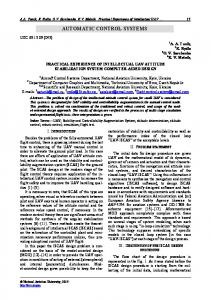
The complementary filter is used to obtain the estimation of a signal out of two redundant information sources [28], which have their origin from different measurements from different transducers (i.e. sensors or detectors). The complementary filter obtains estimation by filtering the signals through complementary networks, which means that if one of the signals is disturbed by high frequency noise, then it is appropriate to choose a low pass filter and consequently obtaining a high pass filter for the other signal. The basic complementary filter is shown in Figure 3.3 where ݔand ݕare noisy measurements of some signal ݖand ݖƸ is the estimate of ݖproduced by the filter. Assuming that ݔhas mostly high frequency noise andy ݔhas low frequency 26
noise, then ܩሺݏሻ acts as low pass filter to filter out the high frequency noise in�ݔ. Therefore ሾͳ� െ �ܩሺݏሻሿ is the complement, i.e., a high pass filter which filters out the low frequency noise in�[ ݕ29]. No detailed description of the noise processes are considered in complementary filtering [30].
�ݕ
ͳ െ ܩሺݏሻ ൌ
߬ݏ ߬ ݏെ ͳ
High-pass
ݖƸ
Fil �ݔ
ܩሺݏሻ ൌ
ͳ ߬ ݏെ ͳ
Low-pass Fil
Figure 3.3 Basic block diagram of the complementary filter.
27
4. Methodology In the following sections the methodology and experimental procedures carried out for modeling and control of the self-balancing vehicle (Elektor Wheelie) are explained in detail.
4.1
System Modeling
Modeling of physical processes is maybe the most important function of Modelica, so the decision of modeling the self-balancing vehicle using a Modelica-based tool such as Dymola was natural. The Dymola environment and the drag and drop block interconnection mode were used for this purpose. Modeling of the Vehicle Body Modeling of any dynamic system is the process of coming up with a set of mathematical equations which rule its physical behavior. In the case of the selfbalancing vehicle, it was decided to obtain a representation of its physical behavior through the use of Modelica’s Multibody library; this library allows the interconnection of mechanical pieces as blocks. A simple model of the self-balancing vehicle was designed through the connection of body boxes, cylindrical bodies, revolute joints and a wheel set. Figure 4.1 shows the resulting model in Dymola.
28
Figure 4.1 Mechanical model of the vehicle’s body. The platform of the vehicle was modeled using two body boxes with the same lengths as the real Elektor Wheelie. On the real vehicle, the platform is a hollow box which accommodates the DC motors used to control the wheels; however, it was decided to model it as a solid block with density 1822.92 Kg/m3; this density value of a box of those lengths corresponds to the total weight of the Elektor Wheelie (35 Kg approximately). The handlebar was modeled as three cylinders with no mass, so they would not affect the model and have been used just for animation purposes. The wheels were modeled using the wheel set block in the Multibody library. The drive of each wheel is determined by an angular velocity reference block. The interaction between the platform and the wheels axis was simulated using a revolute joint, which provides free movement of the platform with respect to the wheel axis mimicking the inverted pendulum behavior. In the specific case of the self-balancing vehicle, the inverted pendulum behavior is dominated by the position of the center of mass of the driver, which was modeled as a 70Kg punct mass at 1m height attached to the center of the wheel axis. In order to allow voluntary movements of the driver whit respect to the vertical position a revolute joint was used. This joint is not a free movement joint but has its angular position driven by an external reference. The ideal angle and angular velocity sensors of Dymola were used for obtaining the three outputs of the system, the angle of the platform relative to the vertical position, the angular velocity and the angular velocity of the wheels.
29
DC Motors Modeling In the self-balancing vehicle, each wheel is driven by a DC motor. In order to design a proper control system, it was necessary for the final model to behave as similar as possible to the real motors; this is why it was important to take some time in order to make a proper identification of the motors. During the identification of the motors, Matlab’s System Identification Toolbox was used to generate a linear model of the DC motors. The identification strategy used was grey box model identification based on a state space representation found in [31]: ௗ
൬ ௗ௧
Ͳ ߮ሺݐሻ ൰ ൌ ቆͲ ߱ሺݐሻ
Ͳ ͳ ߮ሺݐሻ ଵቇ ൬ ቇ ݒሺݐሻ ൰ � ቆ െ ߱ሺݐሻ
(21)
ݕሺݐሻ ൌ ሺͲ ͳሻ ൬
߮ሺݐሻ ൰ ߱ሺݐሻ
(22)
where ߮ሺݐሻ is the angular position of the motor, ߱ሺݐሻ its angular velocity, a and b are physical constants to be determined by the System Identification Toolbox, and ݒሺݐሻ is the voltage input signal. During this project, the input of the motors is not considered to be a voltage signal, but a PWM reference value coming from the microcontroller with values between -180 and 180. The input voltage of the motor is considered to be proportional to this reference, making equation (21) still valid. The input signal used for the model identification was a pseudorandom binary sequence with values -180,180 as it is suggested in [32]. From the registered output signal (angular velocity), several models where generated, these models were compared with data from different experiments; the model which had best fit was selected as the final model. Complete Model of the Self-Balancing Vehicle The final model of the self-balancing vehicle is the model of the vehicle’s body connected with the state space representation of the DC motors. In order to reduce the complexity of the controller, it was decided to use a single model for both motors, thus a single input signal is used in order to stabilize the vehicle. The output signals are those available through sensor measurements in the actual Elektor Wheelie (platform angle relative to the vertical, platform angular velocity and wheel velocity). The connection diagram in Dymola for the final model is shown in Figure 4.2.
30
Figure 4.2 Connection diagram of the final model in Dymola
Model Linearization In order to design a stabilizing controller for the self-balancing vehicle, a linearization of the Dymola model was made around the upright position (ߠ ൌ Ͳ , with non-tilted user). Dymola’s linearization tool automatically chooses the state variables of the mechanical model in order to generate a state space model. During a first phase a state space representation of the vehicle was generated using Dymola; then this representation was reduced with Matlab’s modred. The reduced model was selected to have as states the angular velocity of the platform, its angular velocity and the angular velocity of the wheels (ߠǡ ߠሶǡ )ݓ, assuming the vehicle moves in straight direction, i.e. both motors have the same input. The outputs were chosen to be the same as the states because they are measurements available by sensor readings (accelerometer, gyro and encoders). The reduced model was transformed into discrete form using the c2d command in Matlab with a sampling rate Ts=0.01s which was considered to be enough in order to control the system. For both the Dymola generated model and the reduced model, observability and controlability analysis were performed using the Analysis command of the LinearSystems2 library, also the behavior of both representations was compared in order to establish the validity of the reduced model.
4.2
Control Strategy
A LQR control strategy was used to control the vehicle, and Modelica Linear Systems2 lqr comand was used to get the feedback matrix K. For the selection of matrices Q and R the relative importance of the states and control signal errors were considered. The deviations of ߠ were highly penalized, since keeping a straight position of the platform is the most important job for the controller. The chosen matrices Q and R were: ͳͲͲͲ ࡽൌ൭ Ͳ Ͳ
Ͳ Ͳ ͲǤͳ Ͳ ൱�ǡ ࡾ ൌ ሺͳͲሻ Ͳ ͳͲͲ
31
(23)
Once the matrix K was obtained, the controller was simulated in Dymola. Figure 4.3 shows the block interconnection setup for the closed-loop system simulation. Notice that in order to simulate the model, a world component was used to set the reference system and the direction of the gravity force; additionally the sampler blocks were needed since the K matrix was calculated based on a sampled model. The performance of the controller was tested by simulating diverse behaviors of the user tilt angle.
Figure 4.3 State feedback controller simulation setup.
4.3
Signals and Sensors Processing
On the real vehicle, output signals are acquired using four sensors: two angular position sensors for the velocity of the wheels, an accelerometer for the platform’s tilt angle and a gyroscope for its angular velocity. The sensors are connected to the control unit through its ADC ports. Naturally, the values registered by the microprocessor correspond to voltage values which must be processed according to the unique characteristics of each sensor in order to be interpreted as physical quantities. Wheel Velocity Two angular position sensors (MLX90316) are attached to the wheels of the vehicle, these sensors allowed the measurement of the angular position of the wheel between 00 and 3600. The output of each sensor corresponds to a voltage value which is proportional to the angle position of the wheel. This value is in the range [0.1Vref, 0.9Vref] where Vref is the feed voltage on the sensor. One of the goals of this work was the fixed-point coding, for reasons explained below, it was determined to use an angular scale in the ሾെߨǡ ߨሿ range for angular position. This range is convenient because of its symmetry and the 32
lower modulus compared to the degree scale which lets more variable space to represent the fractional part of the values. Besides, all the variables coming as a result of sensor processing were changed into radian units to ensure consistency. Because of the selection of a symmetric interval, an offset constant has to be considered. This way the angle of the wheel ߮ in a specific moment was calculated as: ߮ ൌ ሺ ݁ݎݑݏܽ݁݉ܥܦܣെ ݐ݁ݏ݂݂ܥܦܣሻ ߙ כ
(24)
where ADCmeasure is the 10-bit integer value registered by the ADC corresponding to the angular position at a specific moment, ADCoffset=546 is the offset constant which transforms the sensor readings into the symmetric interval and ߙ ൌ ǤͳିͲͳݔଷ ݀ܽݎis the proportional constant of the sensor for a 10-bit ADC with reference voltage 5V. As the design of the controller required as an input the angular velocity of the wheels, ߱, it was necessary to implement an estimator which uses as input the calculated angle position. For this purpose a simple difference estimator was chosen. The angular velocity of the wheels is calculated every Ts=0.005s, using the current angle ߮ and the angle during the last reading ߮ௗ as : ߱ൌ
ఝିఝ ்௦
(25)
The angular velocity variable may have positive or negative value, depending on the rotating direction of the wheel; however, erroneous calculations are made when the wheel has it angular position around Ȃ ߨ and ߨ� ݀ܽݎbecause of the characterisctis of the sensor. For example, when the wheel is rotating in the positive velocity direction, a negative velocity could be calculated near the discontinuity region. In order to solve this issue, the direction bit which drives the H-bridges was used as an auxiliary variable. When the sign of the velocity and the wheel direction are inconsistent, a correction is made on the angular difference. Figure 4.4 shows the flowchart of one wheel estimator with its respective difference corrector.
33
Figure 4.4 Flow chart of the angular velocity estimator with angle difference correction. As the controller was designed to have a single angular velocity state, a single estimator was needed. However, it was decided to calculate the angular velocity for the two wheels and then to calculate the wheel velocity state as: ߱ൌ
ఠ ାఠೝ ଶ
(26)
Where ߱ and ߱ are the angular velocities of the left and right wheel respectively. This approximation is useful when the vehicle is not moving straight and the angular velocity of the wheels are different for each wheel. Platform Tilt Angle and Angular Velocity The vehicle has a sensor board with an accelerometer and a gyroscope, used to measure the tilt angle and angular velocity of the platform, respectively. The output signal of the accelerometer consists of a voltage equivalent to an acceleration value which is expressed in Gravity units ሺሻ. That voltage is converted in a register of 10 bits through one of the ports of the analog to digital converter (ADC) of the microcontroller ATmega32. The following expression permits to calculate the value of the input voltage �୧ : �୧ ൌ
ୈେభబౘ౪౩ ൈ౨ ଵଶସ
34
(27)
where ���ଵୠ୧୲ୱ corresponds to the read value of the ADC register, �୰ୣ is the ADC’s reference voltage and the constant ͳͲʹͶ consists of the total of numbers that can be represented with the register of 10 bits. It is necessary to convert the obtained value via ADC to its corresponding acceleration value using the scaling factor. It should be taken into account that the accelerometer has an offset voltage, which corresponds to the output voltage when the surface of the platform is in parallel position to the ground surface, i.e., when the angle is equal to zero. In this way the expression to calculate the acceleration is: ൌ
ౙౙ ିౙౙ
(28)
οȀοୋ
՜ �
�୧ୟୡୡ ՜ � �୭ୟୡୡ ൌ ͳǤͷ�ሾ�ሿ ՜ ��ሺ
��
ሻ ο οୋ
ൌ ͳͶ�ሾ�Ȁሿ � ՜ ��ሺ
��
ሻ
With the acceleration value it is possible to calculate the tilt angle of the platform by using trigonometry. The measured output signal corresponds to the ܺ axis of the accelerometer. Knowing the Gravity value (ͻǤͺ�Ȁ ଶ ) and the ܺ axis component, is enough in order to estimate the tilt angle of the platform in relation to ground surface. The expression that permits calculating the tilt angle Ʌ of the platform is: Ʌ ൌ � ିଵሺ
ି οȀοୋ
ሻ
(29)
This means, Ʌ ൌ � ିଵሺሻ
(30)
In this case, the most important angles to be measured are the ones around the vertical position relative to the platform’s surface. If the platform reaches an angle higher than 30 degrees, the controller will not be able to return the platform to its upright position, therefore, the small angle approximation can be used when the platform is tilted forward or backward at an angle Ʌ (without horizontal acceleration) [33]: �୧ୟୡୡ �Ǥ ο�Ȁο � ൌ �ͳ�ሾሿ��ሺɅሻ (31) �୧ୟୡୡ ՜ �� ο οୋ
ൌ ͳͶ� ቂ
୫
ቃ ՜ ��
where,��ሺɅሻ � ൎ �Ʌ, in radians. The expression (31) is valid while�Ʌ� ൌ � േ�Ɏ�Ȁ�� ൌ � േ�͵Ͳ�͑.
35
On the other side, the output signal of the gyroscope is a voltage proportional to an angular velocity value in degrees per second units. That voltage is converted to a 10-bit value by the ADC using Equation (27). Subsequently the previous value is transformed to its correspondent angular velocity value using the scaling factor and in the same way as in the accelerometer’s case, it is necessary to take into consideration the offset voltage, which is the output voltage when the gyroscope is in steady state. The expression to calculate the angular velocity is: ౝ౯౨ ିౝ౯౨ Ʌሶ ൌ οȀοሶ
(32)
Ʌሶ ՜ ��
�୧୷୰୭ ՜
��
�୭୷୰୭ ൌ ͳǤ͵ͷ�ሾ�ሿ ՜ ���ሺ
��
ሻ� ο οሶ
ൌ ʹሾ�ȀιȀሿ�
In order to obtain the platform’s tilt angle from the angular velocity calculated with Equation (32), first it is necessary to convert units from degrees per second to radians per second, just to be consistent with the units in the system. Secondly, the result of the conversion is integrated in time and in that way the platform tilt angle is obtained. An important requirement to calculate the angle from the angular velocity is that the sample time must remain constant in order to have a correct calculation. Estimation of Platform Tilt Angle Combining the Accelerometer and the Gyroscope In the next sections two approaches which permit the estimation of the platform tilt angle from the combination of the output signals of the accelerometer and gyroscope are presented. Complementary Filter: This type of filter is frequently implemented to obtain a precise value of the platform’s tilt using the data from the accelerometer and gyroscope. In the following section, it is assumed that the acquired measurements from the sensors have been previously converted to the appropriate units by use of the scale factors as explained previously. The accelerometer is a very sensitive sensor and works well in stationary state, i.e., in situations where the horizontal acceleration generated by the platform’s movement is affected by high frequency noise. Therefore, the accelerometer signal (ߠ in Figure 4.5) must pass through a low pass filter, whose purpose is to pass the changes that occur over long periods of time and filter changes that occur over short time intervals. ሶ in Figure 4.5) is a sensor which records zero (sensor’s The gyroscope (ߠ௬ offset) as its output signal when in steady state and is more sensitive when it is rotating, i.e., the gyroscope is less sensitive to the influence of vibration measurements than the accelerometer. Complementary to the case of the accelerometer, a high-pass filter is used, which aims to allow the pass of signals 36
that occur over long intervals of time and filters the ones that are essentially stationary over the course time. After filtering the respective output signals from the accelerometer and gyroscope, these are added together to obtain the final value of the inclination angle �ߠி (Figure 4.5) of the platform.
Figure 4.5 Block diagram of the implemented Complementary Filter It is necessary to consider the time constant of the filter, which refers to the time that the filter will act on each signal. The following expression is used to calculate the time constant [33]: ɒൌ ൌ
ୟ�Ǥୢ୲ ଵିୟ த
�
(33) �
ୢ୲ାத
(34)
The filter coefficient (Equation (34)) is calculated using the time constant (߬) and the sampling period (݀)ݐ. Usually the time constant is less than one second, so it can ensure small variations in the estimated angle. However, it is important to consider that the smaller the time constant the greater the noise in the system due to the horizontal acceleration of the platform. The expression used to estimate the tilt angle using complementary filter has the following structure [33]: Ʌେ ൌ �Ǥ ൫Ʌ୭୪ୢ̴େ Ʌ୷୰୭ Ǥ ൯ � �Ǥ Ʌୟୡୡ where
37
(35)
Ʌେ ՜� Estimated angle by the complementary filter Ʌ୭୪ୢ̴େ� � ՜ Complementary filter's old estimated angle Ʌ୷୰୭ � ՜ Gyroscope measured angle Ʌୟୡୡ � ՜�Accelerometer measured angle ՜� High pass filter coefficient ൌ ሺͳ െ ሻ ՜ Low pass filter coefficient �Ǥ ൫Ʌ୭୪ୢ̴େ Ʌ୷୰୭ Ǥ ൯ ՜�High pass filter applied to the gyroscope's signal ൫Ʌ୭୪ୢ̴େ Ʌ୷୰୭ Ǥ ൯ � ՜� Integration part, which seeks to find the new angle of the platform using the old angle plus the change of angle (angular velocity multiplied by the sampling period) �Ǥ Ʌୟୡୡ � ՜ Low pass filter applied to the accelerometer's signal The design of the complementary filter was performed empirically, i.e. the sample time was chosen so that the filter is executed a total of one hundred times per second and a time constant of 0.05 seconds, to determine the filter coefficient. Using Equation (34) the filter’s coefficient can be calculated: ݀ �ݐൌ ͲǤͲͲͳ�ݏ݀݊ܿ݁ݏ
(36)
߬� ൌ ͲǤͲͷ�ݏ݀݊ܿ݁ݏ
(37)
this results in: Ǥହ
ܽ ൌ ǤହାǤଵ ൎ ͲǤͻͺ
(38)
The filter´s coefficient is the coefficient of the high-pass filter. The chosen value for the time constant indicates the time limit which needs to pass from giving more relevance to the gyroscope’s measurement to giving importance to the accelerometer’s measurement. Therefore, for time intervals of less than 0.05 seconds, the integration of the gyroscope takes higher precedence and the noise due to horizontal acceleration is filtered. For longer periods of time constant, more weight is given to the accelerometer’s measurement. When the filter’s coefficient and the sampling period are inserted in equation (35), the final complementary filter is obtained: Ʌେ ൌ ͲǤͻͺ�Ǥ ൫Ʌ୭୪ୢ̴େ Ʌ୷୰୭ Ǥ ͲǤͲͲͳ�൯ �ͲǤͲʹ�Ǥ Ʌୟୡୡ
(39)
One of the characteristics of the gyroscope which must be dealt with is that it has a deviation in its measurements (drift) while the time passes, i.e. in addition 38
to the offset, therefore, it should be taken into account that the voltage increases as time passes. This results in erroneous measurements of the angular velocity and thus the inclination angle. The effect of the drift in the measurements of the gyroscope is fixed by the complementary filter, because as previously explained, the signal of the gyroscope has higher relevance during time intervals shorter than the time constant. Thus, in greater time intervals the signal of the accelerometer has more relevance for the estimation of the angle. However, in the case of this project, even if the complementary filter was a good way to estimate the tilt angle of the platform, which corresponds to one of the states of the system to be controlled, it was also required to estimate the angular velocity of the platform. While the complementary filter method is able to correct the drift due to the gyroscope in the calculation of the tilt angle, the drift stays present in the estimation of the angular velocity as will be shown later in the results of the experiments. Kalman Filter This filter is used to estimate the tilt angle and the drift of the platform’s angular velocity. Below is a description of the sensor signals through equations. ݏ௬ ൌ ߠሶ ݀ ݓଵ
(40)
ݏ௬ ՜� Gyroscope signal (angular velocity) in ሾ݀ܽݎȀݏሿ ߠሶ � ՜ Real angular velocity of the platform ሾ݀ܽݎȀݏሿ ݀� ՜ Drift of ߠሶ�in ሾ݀ܽݎȀݏሿ ݓଵ � ՜ Noise in the gyroscope signal ݏ ൌ �ߠ ݒଵ
(41)
ݏ ՜� Accelerometer signal (angle) in ሾ݀ܽݎሿ� ߠ� ՜ Real inclination angle of the platform in ሾ݀ܽݎሿ ݒଵ � ՜ Horizontal acceleration of the platform considered as noise The resulting state-space representation of equations (40) and (41) is: ݓଵ െͳ ߠ ͳ ቁ ቀ ቁ ቀ ቁ ݏ௬ ܩቀ ݓቁ Ͳ Ͳ ଶ ݀ ߠ ݏ ൌ � ሺͳ Ͳሻ ቀ ቁ ݒଵ ݀
ሶ Ͳ ൬ߠ ൰ ൌ ቀ ሶ Ͳ ݀
(42) (43)
The signal of the gyroscope was represented as an input and the accelerometer signal as an output; under such representation it is possible to 39
obtain a Kalman filter to estimate the desired states. The gain matrix ࡸ was calculated using the Matlab command lqe given a state space system, the noise covariance of the process (ࡽ) and the noise covariance of the measurements (ࡾ). The noise covariances were chosen empirically, i.e., after several trials with various values taking into account that it should rely more on the gyroscope signal than on the accelerometer’s signal, since equation (41) does not describe all the dynamics of the accelerometer. It is also known that the influence of the gyroscope’s drift is small because it has slow change (ramp behavior) over time. The selected covariance matrices were: ͲǤʹ Ͳ ቁ�� Ͳ ͲǤͺ
ܧሼ ݓ�ݓᇱ ሽ � ൌ ࡽ ൌ � ቀ
ܧሼ ݒ�ݒᇱ ሽ � ൌ ࡾ ൌ ʹ ܧሼ ݒ�ݓᇱ ሽ � ൌ ࡺ ൌ Ͳ ՜ Corresponds to the cross-correlation
(44) (45) (46)
The first element of the covariance ࡽ indicates how the gyroscope’s noise affects the system and the second element indicates how quickly the drift varies. The covariance expresses the size of the accelerometer’s noise, which is the largest value and it means that is expected that this sensor presents a greater noise in the measurements. Then the representation of the Kalman filter was discretized using the Matlab command c2d. Figure 4.6 shows the block diagram of the controller unit with the implemented Kalman filter estimator. In order to test the performance of the Kalman filter as an inclination estimator, it was programmed and tested offline over real data. Once its behavior was proved to be right it was included in the control uint.
Figure 4.6 Block diagram of the implemented Kalman Filter to estimate the tilt angle of the platform and the drift of the gyroscope.
40
Exponentially Weighted Moving Average Filter Naturally, the analog signals coming from sensors were affected by noise, so it was necessary to take special care of those which were not obtained or estimated via complex filters. Specifically, the angular velocity of the wheels and the platform. It was decided to process the control signal in order to avoid spikes which were translated into variations of the wheel velocity which are annoying for the driver. To get smoother signals, an exponentially weighted moving average filter was implemented as: ܵ ൌ
ேିଵ ே
�ܵିଵ ݕ
ݕ ൌ
ௌೖ ே
(47) (48)
The filter requires the storage of a single variable S in order to obtain a smoother representation (yf) of the signal y with N a filter coefficient. It can be easily shown that this implementation corresponds to an exponentially weighted moving average filter with ߙ ൌ ͳȀܰ. This way the filter effect is stronger when N increases. In order to check the behavior of the filter and to determine an optimal value for N, the filter was tested on the actual control unit for different values of the coefficient N.
4.4
Controller Implementation on the Atmega32
Taking into account the characteristics of the self-balancing vehicle, it was natural to view the microcontroller as an embedded system with the single function of providing the stabilizing control. The main goals for the programming of the control unit (Atmega32) were the generation of periodic tasks corresponding to control and estimation tasks as well as the handling of fixed-point representation of floating point variables. The program was structured as a task dispatcher with three different periodic tasks, the controller itself, the wheel estimator (velocity calculator) and the platform estimator (complementary filter or Kalman filter). In order to create a periodic dispatcher one of the timer interrupts in the Atmega32 was used. The 8bit timer (timer 2) was set into top interrupt mode at 15625Hz. By changing the timer counter register TCNT2 it was possible to obtain faster timer interrupts than 1/15625s. It was decided to set the controller execution period to Ts=0.01s which is the sample time set during the design of the controller. The estimators were set to run with Ts=0.005s. The reason that the estimators are running at a higher frequency is that some estimators need certain number of iterations in order to get a reliable estimation, so it is convenient to have them running at a higher frequency. The maximum wheel velocity corresponds to an 11Hz frequency, the frequency of the estimator is much higher so it would not cause sampling problems. The wheel and platform estimators were set to have the same frequency but they are treated as separate tasks, which is useful for future applications if different estimators want to be tested. 41
The interrupt routine is shown in Table 4.1a. The interrupt period was set to Ti=0.005s, this number is convenient as it is possible to get the periods of all the three tasks by using the minimum amount of interrupts. Note that computing tasks are not performed inside the interrupt handler, instead Boolean flags were used to indicate when it is time to perform a certain task, then the computations are performed in the main routine if the corresponding task is ready to be performed (Table 4.1b). Table 4.1 Periodic tasks implementation on the Atmega32 a) Timer interrupt routine … counter_controller++; //auxiliary period variables counter_wheel_estimator++; counter_platform_estimator++; if(counter_wheel_estimator==1){ //Wheel estimator Ts = 0.005 s flag_wheel_estimator++; counter_wheel_estimator=0; } if(counter_platform_estimator==1){ // Platform Estimator Ts = 0.005 s flag_platform_estimator++; counter_platform_estimator=0; } if(counter_controller==2){ // Controller Ts = 0.01 s flag_controller++; counter_controller=0; } TCNT2=0xB1; //set timer counter, interrupts every 0.005s …. b) Dispatcher in main function While(1){ if(flag_controller>0){ … //controller calculations flag_controller=0; } if(flag_wheel_estimator>0){ … // wheel estimators calculations flag_wheel_estimator=0; } if(flag_platform_estimator>0){ … // platform estimator calculations flag_platform_estimatoe=0; } }
In the same embedded system design approach, it was necessary to establish a communication interface between tasks and between a specific task and the hardware. In the case of the control unit, it was necessary to define interfaces between the estimators and the controller since the controller needs the estimated state values in order to perform its own calculations; additionally, interfaces between the controller task and the motors as well as between the estimator task and sensors had to be defined in order to apply the calculated 42
control signal. There is an extra advantage in programming the control unit in such a structure; the program has three blocks which can be replaced by a programmer who knows the interface functions, this way it is easy to experiment with different coding or estimators. The first set of interfaces were those which allow two tasks to communicate with each other. The only shared resources were the variables corresponding to the calculated states, therefore the only interfaces needed were those to write or read these variables. The shared resources were modeled as global variables, the functions set_StateTilt(ߠ), set_StatePlatformVel(ߠ), and set_StateWheelVel(߱) were simple functions which write the corresponding state global variable, while get_StateTilt(ߠ), get_StatePlatformVel(ߠ), and get_StateWheelVel(߱) read the global variable. By using these functions the communication between tasks was not direct (see Figure 4.7). The problem could get more complex if the tasks ran in parallel so programming structures as semaphores or locks would have to be used, however, the implemented program structure did not allow one task to block or interrupt another task, i.e. once a task starts its execution it would not stop until it was finished, so there was not risk of reading wrong values or tasks trying to access the same variable at the same time.
Atmega32 Platform Estimator Ts=0.005s … Calculate platform angle and velocity …. set_StateTilt(ߠ) set_StatelPlatformVel(ߠሶ)
Global variables ߠ ߠሶ
Wheel Estimator Ts=0.005s ... Calculate wheel velocity …. set_StateWheelVel(߱)
߱
Controller Ts=0.01s get_StateTilt() get_StatePlatformVel() get_StateWheelVel() … Calculate control signal
Figure 4.7 Communication between tasks interfaces.
43
The second set of interfaces is formed by those which connect the control unit with the motors and sensors in the vehicle (see Figure 4.8). In order to get the reading from the sensors, four functions are required, corresponding to a simple getADC function call for each sensor. Function set_pwm(char pwm) is basically the interface between the control unit and the motors.
Vehicle Atmega32
Left encoder Right encoder Gyro Acc Left motor Right motor
get_ADCLeftEncoder() get_ADCRightEncoder() get_ADCGyro() get_ADCAdxlA() set_pwm(u)
Figure 4.8 Communication between the control unit and the external hardware It is important to detail set_pwm function separately because it has two main purposes which are vital for the driving of the vehicle. First, it is the function which allows the application of the control signal to the motors and second, it handles the steering instructions. The purpose of the function is to receive a signed value (control signal) and set the PWM duty cycle which drives the motors according to the control signal and the steer direction. In order to turn, the set_pwm function takes information from the steering wheel and adds or subtracts a fixed quantity (10) to each wheel PWM reference value depending on the direction of the turn. When the platform angle is around the upright position the control signal tends to be small and more power is needed in order to turn, consequently a special exception is made when the control signal is small so the turn quantity is changed to 30 (see Table 4.2 a). In order to drive the motors the timer 1 in the Atmega32 was set to work in PWM phase correct mode, the value written in registers OCR1A and OCR1B determines the duty cycle of the input square wave signal of the left and right motors, the smaller the written value the higher the duty cycle and therefore the higher the speed. It is important to notice that the OCR1A and OCR1B do not admit negative values. The effect of a negative control signal (backward movement) is achieved through setting the H-bridge input bit which inverts the PWM coming from the control unit.
44
Table 4.2 Set_pwm function. a)Steer correction. b) Set motors velocities a) set_pwm function (steer handling) void set_pwm(short pwm){ short set=0; //auxiliary variable char dir=0; //wheel direction char turn=0; //steering wheel direction short right=0; //auxiliary right wheel variable short left=0; //auxiliary right wheel variable turn = steering(); //get steering direction if(turn==1){ //no turn right=pwm; left=pwm; } if(turn==0){ //turn left if(pwm>=0){ //when fordward if(pwm=0){ //when forward if(pwm>(na+nb-nc) if (temp32767) c=32767; else c=temp;
The second step while coding in fixed-point is to determine the proper Qm.n format for each variable and constant. For this, a rule was set for all variables: the format was chosen so the minimum amount of integer bits are used to represent the maximum value a variable can adopt, the rest of the bits are assigned to the fractional part of the variable. The minimum and maximum values for each measured variable were measured in extreme conditions in order to make sure the variable size could handle movements even outside the typical use range. A special consideration was taken with the control signal since it is a PWM value (dimensionless) which can adopt values between 0-255 in integer form (safely 46
limited to 180 by the set_pwm(u) interface), Therefore no fractional part was assigned to the variable; the same consideration was taken for all integer constants. Table 4.4 shows the chosen Q format for the three main states and the control signal, any intermediate variable was chosen accordingly in order to maintain coherence of the representations. Table 4.4 Fixed-point format selection for main variables Variable
Range
Q format
Fixed-point range
Precision
Wheel angular velocity ߱
[-70,70] rad/s
Q7.8
[-128,127.9960] rad/.s
3.906x10⁻³ rad/s
Platform angle ߠ
[-1,1] rad
Q1.14
[-2,1.999] rad
5.103x10⁻⁵ rad
Platform angular velocity ߠሶ
[-3.5,3.5] rad/s
Q2.13
[-4,3.999] rad/s
1.220x10⁻⁴ rad/s
Control signal u
[-180,180]
Q15.0
[-32768,32767]
1
The wheel velocity estimator as well as the controller (K gain) were programmed using fixed-point representation. The complementary filter and the Kalman filter as estimators for the platform states were programmed separately; the two implementations were tested in order to compare the performance between the two estimators.
4.6
Automatic fixed-point code generation using Dymola
The Modelica_EmbeddedSystems library provides an environment to design and simulate embedded systems based on the treatment of complex systems as separated tasks and subtasks which interact together or with tasks or subtasks on other targets. The library provides the tools to set time and type parameters for each task, simulate different kinds of communication and interfaces between tasks, as well as features to automatically generate code for external targets. Task separation in Dymola The Modelica_EmbeddedSystems library bases its operation on the fact that complex systems can be separated into smaller tasks; special configuration blocks are included for this purpose. For each simulation it was necessary to specify the characteristics of the targets where the tasks are running. In order to evaluate the self-balancing vehicle as an embedded system, the model was tested using the separation in tasks (Figure 4.9).
47
Figure 4.9 Embedded system model simulation setup The system formed by the simple gain feedback and the vehicle model was divided in two tasks, one for the controller and one for the vehicle mechanics. Each task has a subtask, these are actually the controller and the model. The controller and the model were chosen to be executed on different targets, the controller on a fixed-point target, which allowed the simulation of the fixed-point resolution effects on the control of the vehicle, and the model on the dymosim (Dymola’s simulation) target. The model was set to be a continuous subtask while the controller was periodic with Ts=0.01s, which matched the selection made during the design process. In order to simulate the partitioning of tasks, the Modelica_EmbeddedSystems library has special communication blocks; 48
CommunicateReal (also equivalent blocks are used for integer or Boolean communication) is the main block which partitions the scope of each task as well as the communication types or parameters between tasks (Figure 4.10).
Figure 4.10 CommunicateReal block configuration window The ComminicateReal block has the ability of setting the type of communication as communication between tasks, between subtasks, between parts of the same task (simple wire) and from/to external ports. The communication between tasks and subtasks type has features to simulate quantization and delays in AD/DA converters. This mode was used during the simulations in order to separate between the control task and the actual vehicle. During the automatic code generation, the most important communication types handled by the block are to/ from port communication types; these allow the inclusion of code in order to emulate external communication interfaces. These types of communication were used during the automatic code generation because they allowed a direct mapping to the programmed interfaces in the control unit; this will be further explained in the following sections. Besides defining the communication “rules” the block permits to partition tasks or targets as it keeps the specifications of its input and output task. Code generation In order to automatically generate code, preparations had to be made. First, it was necessary to create a mapping between the Modelica variables and the C functions programmed as interfaces in the main program structure. This was achieved by using Modelica mapping functions, which were programmed as functions that map an external C code line corresponding to an interface call in the control unit base code. In order to use the mapping functions, it was necessary to create a to/from port communication block which could be used as communication type in the CommunicateReal block. 49
The interfaces which have the function of writing variables or obtaining information from a task extended the PartialReadRealFromPort class; the interfaces whose function is to send information to a task extended the PartialWriteRealToPort. Using these conventions it was possible to set the task separation using Dymola in the same way it was structured on the base program of the control unit. Table 4.5 and Table 4.6 show an example of the mapping procedure for the set_pwm(u) (write interface) and get_StateWheelVel() (read interface) interfaces. Note that the PartialWrite/ReadTo/FromPort block has as only function calling a Modelica function which calls the interface in the control unit code. The function call must have an extra time parameter in order to work properly and since void functions are not supported, the writing interfaces required a dummy variable which acted as a fictitious output. Table 4.5 Configuration of communication port for set_pwm interface a) To port block block set_pwm extends Modelica_EmbeddedSystems.Interfaces.BaseReal.PartialWriteRealToPort(minValue=180, maxValue=180); protected Real dummy(min= 0, max = 10); equation dummy = Segway.ExternalC.Motor.set_pwm(integer(u),time); end set_pwm; b) set_pwm mapping function function set_pwm input Integer u "PWM value for duty cycle"; input Real Time; output Real dummy; external "C" set_pwm(u); end set_pwm;
Table 4.6 Configuration of communication port for get_StateWheelVel interface a) From port block block get_StateWheelVel extends Modelica_EmbeddedSystems.Interfaces.BaseReal.PartialReadRealFromPort(minValue=100, maxValue=100); equation y = Segway.ExternalC.Wheels.get_StateWheelVel(time); end get_StateWheelVel; b) get_StateWheelVel mapping function function get_StateWheelVel "Get Wheel Angular Velocity" input Real Time; output Real signal; external "C" signal = get_StateWheelVel(); end get_StateWheelVel;
50
Once all the interfaces were redesigned in Dymola, the controller and estimators were coded in Modelica. In order to use the automatic fixed-point code generation it was necessary to give additional information about the range of certain variables as well as the desired fixed-point resolution. This was possible by modifying the range attributes of variables and using annotations. By modifying the min and max attributes of the variable it was possible to set the number of bits representing the integer part of the variable and through the fixedpoint annotation it was possible to set the number of bits used to represent its fractional part (Table 4.7). Table 4.7 Range attributes and annotations for main variables. Variable
Range
Q format
Annotation
Wheel angular velocity ߱
[-70,70] rad/s
Q7.8
(min=-70,max=70)annotation(fixedpoint(bits=8))
Platform angle ߠ
[-1,1] rad
Q1.14
(min=-1,max=1)annotation(fixedpoint(bits=14))
Platform angular velocity ߠሶ
[-3.5,3.5] rad/s
Q2.13
(min=-3.5,max=3.5)annotation(fixedpoint(bits=13))
Control signal u
[-180,180]
Q15.0
(min=-180,max=180)annotation(fixedpoint(bits=0))
Each programmable block in the control unit (controller and estimators) was programmed as a Modelica block. The programmable blocks could be designed by interconnecting blocks from the Moleica Standard libraries, but this could bring two problems. First, the fixed-point code generation does not support function calls so, for example, a limiter could not be used since it calls smooth function; additionally, the interconnection of multiple blocks tends to generate a greater number of intermediate variables which makes the analysis of the generated code more difficult. Table 4.8 shows the code for the controller block in Modelica, the annotations and modifications of the variable’s attributes are made when each variable and constant are defined. Similar blocks were created for the wheel velocity estimator and the two different platform angle and velocity estimators.
51
Table 4.8 Modelica block for the state feedback controller Code in Dymola of the state-feedback controller block Controller extends Modelica.Blocks.Interfaces.BlockIcon; Modelica.Blocks.Interfaces.RealInput PlatVel(min=-3.8,max=3.8) "Connector of Real input signal"annotation (fixedpoint(bits=13)); Modelica.Blocks.Interfaces.RealInput PlatAng(min=-0.9,max=0.9) "Connector of Real input signal 2"annotation (fixedpoint(bits=14)); Modelica.Blocks.Interfaces.RealInput WheelVel(min=-70,max=70) "Connector of Real input signal"annotation (fixedpoint(bits=8)); Modelica.Blocks.Interfaces.RealOutput Control(min=-200,max=200) "Output signal connector" annotation (fixedpoint(bits=0)); discrete Real Sum(min=-32000,max=32000) annotation(fixedpoint(bits=0)); discrete Real Maf(min=-200,max=-200) annotation(fixedpoint(bits=0)); discrete Real Control1(min=-200,max=200) annotation(fixedpoint(bits=0)); parameter Real K1=8.9552 annotation(fixedpoint(bits=10)); parameter Real K2=278.994 annotation(fixedpoint(bits=5)); parameter Real K3=89.2559 annotation(fixedpoint(bits=7)); parameter Real K1maf(min=0, max=1) = 0.9 annotation(fixedpoint(bits=15)); parameter Real K2maf(min=0, max=0.2) = 0.1 annotation(fixedpoint(bits=15)); equation when sample(0,0.1) then Control1=K1*WheelVel+K2*PlatAng+K3*PlatVel; Sum = (K1maf * pre(Sum)) + Control1; Maf = Sum * K2maf; end when; Control=Maf; end Controller;
As the main program in the control unit had three programmable tasks, the code for each one was generated separately. In order to do this a simulation setup was set for each block; Figure 4.11 shows the setup for the state feedback controller. The communicateReal blocks had the purpose of defining the interfaces for the tasks. In the state feedback controller four communication interfaces were needed: three from port communication type blocks corresponding to get_StatePlatfotmVel, get_StateTil and get_StateWheelVel and one to port corresponding to set_pwm interface. As the corresponding Modelica mapping functions were designed to make a call to the actual interfaces in the control unit, it was expected to get a simple function call in the generated code for every communicateReal block in the simulation setup. The task to be automatically generated was set to be executed at an external fixed-point target type (the actual vehicle). This way Dymola generated fixed-point code which could be pasted into the main structure of the control unit. A final consideration had to be made in order to achieve the code generation: the simulation would not run unless the simulated model had a first order differential equation in it. As the tasks did not have any differential equation, the equation der(x)=-x was included in all the 52
models for code generation, this had no effect in the regular calculations of the tasks.
Figure 4.11 Setup for the state feedback controller code generation Once a block was simulated, Dymola generated a C file containing all the variable and constant declarations in fixed-point representation (declarations.c file) and another one containing the match calculations in fixed-point (equations.c file). Similar setups were implemented for each one of the three tasks in the control unit. The generated codes were analyzed searching for any fault, modified when necessary and then tested in the actual vehicle through test rides in order to evaluate the performance of the controller.
4.7
Real-Time Communication
The performance of the Modelica_EmbeddedSystems library for real-time applications was tested by designing a simple application which would allow bidirectional communication in real time between the vehicle and Dymola. For this, previously designed by Dassault Systemes add-on packages (CommunicationMSWindows and Lego_Mindstorms) were used as basis for keyboard handling and Bluetooth communication. The designed application consisted in controlling turns and forward movements of the vehicle using the keyboard arrows when no one was riding it, while receiving signals from the vehicle for real-time plotting. The exchange of data was established between a computer with Bluetooh capability and a Bluetooth to serial converter on the vehicle. Control Implementation Aspects The base program on the control unit had to be modified in order to be able to change between modes and to receive and handle instructions from the computer. Two main aspects had to be considered, first the control aspect and second the communication instructions.
53
The physical design of the vehicle makes its center of mass to be slightly inclined forward with respect to the platform’s vertical position when no rider is driving it. This resulted in a permanent trend of the vehicle to lean forwards and consequently an acceleration of the wheels causing the vehicle to move forward permanently. As it was desired that the vehicle was stable, even when no rider was on it, a way to avoid the effect of the tilted center of mass had to be created. Figure 4.12 shows the implemented alternative. The code was modified in order to include a reference ߠ for the platform angle; this implementation solved two problems at the same time, the permanent leaning of the platform was eliminated by setting a negative angle reference which corresponded to the angle of the platform when the center of mass of the chassis was in a vertical position, and the remote control of forward movements was achieved by setting an angle reference value slightly higher than the reference when still.
Figure 4.12 Modified control structure in order to follow references on the inclination angle of the platform The addition of a reference and the difference on the dynamics when a rider is on the vehicle compared to when no rider is on it brought more implementation issues. It was necessary to decide when and how a reference switch had to be made. Additionally, a less aggressive controller was needed during the no rider mode, and it was necessary to define when and how to do the switching. A Statechart defining the algorithm for switching controller and angle reference is shown in Figure 4.13. The controller is changed when the user rides the platform, this event is registered by the controller unit as a signal which comes from a foot switch on the platform. When a rider is on the platform, the angular reference corresponds to a horizontal angle of the platform (Foot reference= 0 rad), when there is no rider two angular references for the platform are possible, a negative reference for compensating the inclined center of mass of the chassis (Stop reference) which is switched to a slightly higher reference (Forward Reference) value when a signal from keyboard is received. 54
Figure 4.13 Controller and reference switching Statechart. The Statechart in Figure 4.13 defines the events that trigger the change of controllers and reference values, but does not specify the structure of the actual changes in the variables. A change in the reference value is a simple step function. The typical behavior of a step function as reference produces a large control signal which could result in the vehicle leaving the linear zone where the model used is valid. A second practical consideration must be made in the particular case of the self-balancing vehicle: when the vehicle is standing by itself, the angle reference is a negative value. At the moment the user rides the platform the reference value changes to zero. If that change had a step shape the vehicle would sharply accelerate backwards and hit the user’s leg. In order to avoid sharp changes in the control signal when changing references, the actual reference which enters the system ߠ was calculated as: ߠೖ ൌ ͲǤͻͻʹߠ
ିଵ
ͲǤͲͲͺߠ௪
(49)
Where ߠ௪ is the final angle value of the platform. The equation represents a filter which generates a smooth and slower response than a step response. In a similar approach, a less aggressive controller was intended to run when no user was on the vehicle; the controller was designed to be a state feedback gain with different gain matrix. This change of parameters of the gain matrix could also result in a sharp change of the control signal. The solution for a bumpless change of matrix K in the controller was similar to the one applied to the reference changes: ࡷ ൌ ͲǤͻͻʹࡷିଵ ͲǤͲͲͺࡷ௪
55
(50)
Dymola Implementation Aspects In order to send and receive data from and to the computer, elements in the CommunicationMSWindows and Lego_Mindstorms packages (Modelica_LinearSystems library add-on packages) were used. The setup of the program is shown in Figure 4.14.
Figure 4.14 Communication program setup in Dymola The program was divided into two tasks, one executed in the vehicle and one executed in the computer. The task executing in the vehicle received information from the computer regarding the remote controlling, and sent the three states and the control signal via Bluetooth. The definition of this task is purely theoretical as it does not affect the simulation, in fact the interfaces of the vehicle tasks could be programmed as dummies. The task executing in the PC received the four signals and sent remote control instructions from the keyboard. The keyboard controller is based on the keyboard features in the CommunicationMSWindows, and was set to get information from the keyboard every 0.1s and set the output as shown in Table 4.9. The control unit was programmed to translate the output values of the keyboard function into left, right and forward movements, combinations of the above and no movement, when a user was not riding the vehicle.
56
Table 4.9 Keyboard block function Up Key 0 0 0 0 1 1 1 1
Left Key 0 0 1 1 0 0 1 1
Right Key 0 1 0 1 0 1 0 1
Output 0 -3 3 0 1 -2 4 1
The communication interfaces are based on the Lego_Mindstorms add-on package. The Bluetooth configuration block did not need to be modified, its function is calling external functions in order to open the COM port in the computer at the beginning of the simulation and close it at the end. On the other hand, the interfaces to send and receive data via Bluetooth had to be modified in order to set them as periodic tasks such that the task wrote the keyboard information on the computer’s COM port and read the four data blocks from the port every 0.1s. Coherency Between Dymola and the Control Unit The program in the control unit had to process and interpret the data sent by Dymola as well as send four information blocks. In order to do this a synchronization and communication protocol between the PC and the control unit needed to be created. The Bluetooth interfaces were defined such that an information block contains six bytes organized as shown in Figure 4.15. The two first bytes were used as synchronization bytes and the other four bytes corresponded to the 32 bit number to write on the port sent from least significant byte to most significant byte. The variables in the controller had 16 bit size so DATA2 and DATA3 in the information block were set to 0x00 or 0xFF depending on whether the variable to send was positive or negative.
0x04
0x00
DATA0 DATA1 DATA2 DATA3
Figure 4.15 Information block for Bluetooth communication In order to achieve synchronization between Dymola and the control unit the Rx interruption on the Atmega32 was used. Each time Dymola sent an information block (every 0.1s), the program in the control unit processed the remote control commands and sent back four information blocks containing the state and control signals (Figure 4.16).
57
Rx interrupt?
No
Yes Read incoming block
Correct package?
No
Yes Get remote control direction
Send State Wheel velocity package Send State Platform angle package Send State Platform angular velocity package Send Control signal package
Figure 4.16 Data handling in the control unit.
58
5. Results and Analysis This chapter presents the experiments and results obtained during the course of this project. Each section describes the results and compares them with simulations where deemed necessary.
5.1
Mechanical Model
Figure 5.1 shows the 3D model visualization of the two-wheeled self-balancing vehicle when it is animated in Dymola. The simulation was setup using components in the MultiBody library as previously shown in Figure 4.1. The driver is visualized as a point mass which dominates the inverted pendulum behavior.
Figure 5.1 Two-wheeled self-balancing vehicle 3D model visualization in Dymola In order to test the behavior of the vehicle, the simulation was run with a small initial lean angle of the driver. As it is shown in the Figure 5.2, when the user mass leans forward, the vehicle starts to fall to the front pivoting over the wheel axis and consequently increasing the platform angle. Since there is no simulated floor or solid ground, the vehicle keeps falling describing a pendulumlike movement. The vehicle behaves as an inverted pendulum when it is not controlled being impossible to keep it in upright position.
59
Figure 5.2 Behavior of the platform angle when the user leans forward and the vehicle does not have a controller
5.2
Motor Identification
In order to get a linear model of the motors, a pseudo-random binary sequence in the range [-180,180] was used as PWM input signal, the output was chosen to be the angular velocity of the wheels (Figure 5.3). The vehicle had its wheels rolling in the air during the test. Using the System Identification toolbox in Matlab, three different models were generated. A two-step input signal was used in order to compare the performance of the models against the response of the actual motors (Figure 5.4). The chosen model was the one which best fitted the real response (89.58%): ௗ ௗ௧
൬
߮ሺݐሻ ߮ሺݐሻ Ͳ ͳ Ͳ ൰ൌቀ ቁ൬ ൰ �ቀ ቁ ݒሺݐሻ ߱ሺݐሻ Ͳ െͳʹǤͻʹͺ ߱ሺݐሻ ʹǤͺͻͶ ݕሺݐሻ ൌ ሺͲ ͳሻ ൬
߮ሺݐሻ ൰ ߱ሺݐሻ
[3.1]
[3.2]
During a first approach it was considered to obtain a model for each motor. However, some previous experiments showed that both motors had very similar responses so it was simpler and accurate enough to use a single model for both motors.
60
Figure 5.3 PWM value input and angular velocity used during the motors identification.
Figure 5.4 Response of the actual motor and generated models to a given input signal.
61
5.3
Linear Model
The motor model was connected to the mechanical model in Dymola. Using the linearize command the obtained state space model of the vehicle was: ݔଵሶ Ͳ ݔଶሶ Ͳۇ ۊ ۇ ݔሶ ۈଷ Ͳۈ ۋ ݔ ۈସሶ Ͳۈ ۋ ݔ ۈହሶ Ͳۈ ۋ ݔ ۈሶ Ͳۈ ۋ ݔ ۈሶ ۋൌ Ͳ ۈ ݔ ۈሶ ۋ Ͳ ଼ ݔ ۈሶ ۈ ۋ Ͳ ۈ ଽ ۋ ۈ Ͳ ݔ ሶ ۈ ۈଵ ۋ ݔۈଵଵሶ Ͳۈ ۋ Ͳ ݔଵଶሶ ݔۉଵଷሶ Ͳۉ ی
Ͳ Ͳ Ͳ Ͳ Ͳ Ͳ Ͳ Ͳ Ͳ Ͳ Ͳ Ͳ Ͳ
Ͳ Ͳ Ͳ Ͳ Ͳ Ͳ Ͳ Ͳ Ͳ Ͳ Ͳ Ͳ Ͳ
Ͳ Ͳ Ͳ Ͳ Ͳ Ͳ Ͳ Ͳ Ͳ Ͳ Ͳ Ͳ Ͳ
Ͳ Ͳ Ͳ Ͳ Ͳ Ͳ Ͳ Ͳ Ͳ Ͳ Ͳ Ͳ Ͳ
ͲǤͳͲʹͷ ͲǤͳͲʹͷ Ͳ Ͳ Ͳ Ͳ Ͳ Ͳ Ͳ Ͳ Ͳ Ͳ Ͳ Ͳ െͲǤ͵ʹ ͲǤ͵ʹ Ͳ Ͳ Ͳ Ͳ Ͳ ͳ Ͳ Ͳ Ͳ Ͳ Ͳ Ͳ Ͳ ͳ Ͳ Ͳ Ͳ Ͳ Ͳ െ͵ͳͶǤʹ Ͳ Ͳ Ͳ Ͳ Ͳ Ͳ Ͳ െ͵ͳͶǤʹ Ͳ Ͳ Ͳ Ͳ Ͳ Ͳ Ͳ Ͳ ͳ Ͳ Ͳ Ͳ ͵ʹǤͲͶ ͵ʹǤͲͶ ͻǤʹ Ͳ ͳͷͺͻͲͲ ͺͺǤͻ Ͳ Ͳ Ͳ Ͳ Ͳ Ͳ ͳ Ͳ Ͳ Ͳ Ͳ Ͳ െͳͷͻͲͲ െͻʹǤʹ Ͳ Ͳ Ͳ Ͳ Ͳ Ͳ Ͳ Ͳ Ͳ Ͳ Ͳ Ͳ Ͳ Ͳ Ͳ
ݕଵ Ͳ Ͳ ൭ݕଶ ൱ ൌ ൭Ͳ Ͳ ݕଷ Ͳ Ͳ
Ͳ Ͳ Ͳ Ͳ Ͳ Ͳ
Ͳ Ͳ Ͳ ͳ Ͳ Ͳ
Ͳ ͳ Ͳ Ͳ Ͳ Ͳ
Ͳ Ͳ Ͳ Ͳ ͳ Ͳ
Ͳ Ͳ Ͳ
ݔଵ Ͳ Ͳ ݔଶ Ͳ Ͳ ۇ ۊ ݔ ۇۊ ۊ Ͳ ଷ Ͳ ۈ ۋ ݔ ۈۋ ۋ Ͳ ସ Ͳ ۈ ۋ ݔ ۈۋ ۋ Ͳ ۈۋହ ۋ Ͳ ۈ ۋ ͵ͳͶǤʹ ۋ Ͳ ۈ ۋ ݔ ۈ ۋ ͵ͳͶǤʹ ۋ ݔ ۈ ۋ ݑ ۋ Ͳ ۈ Ͳ ۋ Ͳ ۈ ۋ ଼ݔ ۈ ۋ െͶǤͲͻݔ ۈ ۋଽ ۋ Ͳ ۈ ۋ Ͳ ݔۈ ۋଵ ۋ Ͳ ۈ ۋ Ͳ ݔۈ ۋଵଵ ۋ Ͳ ۈ ۋ ݔଵଶ Ͳ ͳ െͳʹǤͻ͵ݔۉ یଵଷ ʹۉ یǤͺͻͶی
Ͳ Ͳ Ͳ Ͳ൱ ݔ Ͳ Ͳ
The input is the PWM signal, the outputs are the platform angle, the wheels velocity and the platform angular velocity. The states were automatically selected by Dymola and are shown in Table 5.1. Table 5.1 States of the linear model State x1 x2 x3 x4 x5 x6 x7 x8 x9 x10 x11 x12 x13
Physical variable x axis position of the vehicle y axis position of the vehicle Angle of the wheel axis from the x axis Left wheel angle Right wheel angle Left wheel velocity Right wheel velocity Platform angle Platform angular velocity User angle User angular velocity Motor angle Motor angular velocity
62
Figure 5.5 Open loop generated model pole-zero map Through the pole-zero map (Figure 5.5) it is possible to determine that the generated model is not stable, since it has one pole in the right semi-plane and six poles in zero. Moreover, the Analysis command in Dymola shows that the system is not controllable and not observable. A reduced-order model was needed in order to reduce calculations and to get a controllable and detectable representation. A reduced order system, taking the outputs as states is given by: ߠ Ͳ ሶ ൱ ൌ ൭ͻǤʹ ൭ ߠ ௗ௧ Ͳ ߱ ௗ
ߠ ͳ Ͳ Ͳ Ͳ ͵ʹǤͲʹ ൱ ൭ ߠሶ ൱ ൭െǤͲͺ൱ [ ݑ3.1] Ͳ െ͵ͳ͵Ǥͻ ߱ ͻǤͶ͵
ݕଵ ͳ ൭ݕଶ ൱ ൌ ൭Ͳ ݕଷ Ͳ
Ͳ Ͳ ߠ ͳ Ͳ൱ ൭ ߠሶ ൱ [3.2] Ͳ ͳ ߱
This reduced representation is not stable because it has one pole in the right semi-plane (Figure 5.6), but it is controllable (and stabilizable) and observable (and detectable). This representation is more convenient because a controller and observers could be used. The dominant poles of the system remain the same so the behavior was expected to be similar.
63
Figure 5.6 Open loop reduced model pole-zero map The controller sample frequency must be at least twice the frequency of the dominant pole (3.12rad/s) and much smaller than the PWM frequency (16MHz), then the chosen value Ts=0.01s is valid. The gain matrix for the sampled system is: ࡷ ൌ ሾെʹͺǤͻͻͶǡ െͺͻǤʹͷͷͻǡ െͺǤͻͻͷʹሿ [3.5] The open loop sampled system pole-zero map is shown in Figure 5.7, the closed loop is shown in Figure 5.8. Note that the closed loop system has all its poles inside the unit circle.
64
Figure 5.7 Open loop sampled model pole-zero map
Figure 5.8 Closed loop sampled model pole-zero map
65
5.4
Controller Simulations
The controller was implemented in Dymola using the configuration in Figure 4.3, and two simulations were tested. In order to test the disturbance rejection of the closed loop system, a disturbance in the platform angle was set to act at time zero. Figure 5.9 shows the behavior of the three outputs when the disturbance acts; the velocity of the wheels increases because of the positive initial platform angle, making the vehicle to move forwards until the platform reaches the upright position to finally decrease progressively to set the three outputs to zero.
Figure 5.9 Output response when the platform has 0.1rad initial angle The second test simulated the behavior during a regular ride; the user stays tilted to the front for the first four seconds of simulation and then straightens. The angle of the user causes an increase in the platform angle and a positive velocity of the wheels while the user is tilted. When the user straightens the system recuperates until the vehicle stops (Figure 5.10). This is the expected behavior for a forward movement of the vehicle when the user is driving it.
66
Figure 5.10 Output behavior during forward ride
5.5
Wheel Velocity Calculation
The wheel velocity calculator was programmed in the control unit and tested using a square wave input. The measurements were highly affected by noise having up to 5rad/s variations when the wheel velocity was constant. It was necessary to filter the signal in order to get a smoother input for the controller. The wheel velocity signal was passed through three exponentially weighted moving average filters with different values of N. Figure 5.11 shows the performance of the programmed filters. The filters introduce a delay on the signal, so the selection of the parameter N was a compromise between smoothness of the response and its velocity. The chosen filter has N=10 and provides a smooth response with a 0.2s delay.
67
Figure 5.11 Exponentially weighted moving average filter response for different N values.
5.6
Platform Estimators
Complementary Filter The complementary filter was programmed in the control unit. The test was to tilt and move the platform of the vehicle and register the inputs and outputs of the complementary filter. Figure 5.12a shows the measurements of the accelerometer. During the last seconds of the test the platform was horizontally accelerated producing noise in the accelerometer. The gyroscope signal (Figure 5.12b) is affected by the time variant offset (drift). At the beginning of the test its value in steady state is zero, and a hundred seconds later this value has increased to 0.1rad/s. The programmed complementary filter output is presented together with a simulated output in Figure 5.12c. In both cases the complementary filter removes the high frequency noise in the accelerometer signal and the effect of the gyro drift in the output angle.
68
Figure 5.12 Complementary Filter performance. a) Accelerometer angle. b)Gyro angular velocity. c) Complementary filter estimated angle.
Kalman Filter: Kalman estimator state space in continuous time: ܮൌ ሺͳǤͳͺ͵ െͲǤ͵ʹͷሻ்
[3.6]
� ݏ௬ ሶ െͳǤͳͺ͵ െͳ ߠ ͳ ͳǤͳͺ͵ ቁ൬ ൰ ቀ ቁቀ ݏቁ ቆߠ ቇ ൌ ቀ ͲǤ͵ʹͷ Ͳ Ͳ െͲǤ͵ʹͷ ݀መ ݀መሶ
[3.7]
ͳ Ͳ ߠ ࢟ ൌ�ቀ ቁ൬ ൰ Ͳ ͳ ݀መ
The continuous-time Kalman filter has a pair of poles at -0.584±0.54j. The sample time 0.005s is much faster than the system therefore it is suitable for sampling the system: ݏ௬ ሶ ͲǤͻͻͶʹ െͲǤͲͲͶͻͺͷ ߠ ͲǤͲͲͶͻͺͷ ͲǤͲͲͷͺ͵ʹ ቁ൬ ൰ ቀ ቁቀ ݏቁ ቆߠ ቇ ൌ ቀ ͲǤͲͲ͵ͳͷ͵ ͳ Ͳ െͲǤͲͲ͵ͳͷ͵ ݀መ ݀መሶ
[3.8] ͳ Ͳ ߠ ࢟ ൌ�ቀ ቁ൬ ൰ Ͳ ͳ ݀መ
The sampled system was programmed in the control unit and tested in a similar experiment as the one carried out for the complementary filter. Figure 5.13a and Figure 5.13b show the accelerometer angle and gyro angular velocity. The most important feature of the Kalman filter is the gyro drift estimation. In 69
order to test this feature, the data was taken several minutes after the moment the filter started to act giving time enough for the drift to reach 2rad/s. The outputs are presented in pairs, the actual output from the control signal and a simulated output given real inputs. Figure 5.13c shows the estimated drift signal, the signal mimics the offset in the gyro signal. Figure 5.13d shows the estimated platform angle, the effects of the accelerometer noise and gyro drift are removed in the same way as the complementary filter. The simulated outputs take about 5s to converge to the actual values of the estimated signals, this happened because the filter had zero initial conditions. In the actual filter the convergence time is smaller because the drift tends to be a near zero value, taking less time for the output to converge. The estimated drift value is subtracted from the value of the angular velocity of the platform in order to get a proper measurement of the state, the Kalman filter is an improved solution compared to the complementary filter since it provides estimated outputs from both states (angle and angular velocity).
Figure 5.13 Kalman Filter performance
5.7
Automatic Code Generation
The controller and estimators codes were automatically generated by Dymola. The C codes were analyzed and modified in order to fit the programming requirements of the compiler and microcontroller. Two files were generated for each estimator and two files for the controller code; the first file contains the variable declarations and the second file contains the equations. The declarations file is divided in two blocks, first a definition of the type variables is made and then the declarations are presented. The type definitions must be changed depending on the compiler used, in this case the int_16 and int_32 types had to be modified as shown in Table 5.2, the int_64 type was removed as such a large variable was not needed in the program. The second 70
block of the declarations file contains the declared variables with a detailed comment which contains the real value of the variable and the Q representation used, this makes easier the evaluation and reading of the code; automatically generated declarations for the controller coefficients are shown in Table 5.3. Table 5.2 Type definitions in automatically generated code a) Type definitions for fixed-point data types generated by Dymola #ifndef DYMOLA_FP_TYPES #define DYMOLA_FP_TYPES typedef char bool_8; typedef char int_8; typedef short int int_16; typedef int int_32; typedef long long int int_64; #endif b) Type definitions for fixed-point data types modified /* Type definitions for fixedpoint data types */ #ifndef DYMOLA_FP_TYPES #define DYMOLA_FP_TYPES typedef char bool_8; typedef char int_8; typedef short int_16; typedef long int_32; #endif
Table 5.3 Controller variables declaration in automatically generated code Gain matrix K variable declarations /* parameter Real controller.K1 = 8.9552 annotation(fixedpoint(bits = 10.0));*/ int_16 controller_K1_FP = 9170; /* Q[5, 10] Derived: min = 17.9104, max = 17.9104 */ /* parameter Real controller.K2 = 278.994 annotation(fixedpoint(bits = 5.0));*/ int_16 controller_K2_FP = 8927; /* Q[10, 5] Derived: min = 557.988, max = 557.988 */ /* parameter Real controller.K3 = 89.2559 annotation(fixedpoint(bits = 7.0));*/ int_16 controller_K3_FP = 11424; /* Q[8, 7] Derived: min = 178.5118, max = 178.5118 */
The equations file is typically divided in four blocks, first the input interfaces are called, then the calculations are performed, next the output interfaces are called and finally the variables are updated. The interfaces calls are mapped to the CommunicateReal block configuration depending on if a from port or to port communication type is selected. Table 5.4 shows the file structure in the controller case, first the three states are accessed via the get_State interfaces, then the control signal is calculated, the control signal is applied to the motors via set_pwm interface and finally a filter variable is updated.
71
Table 5.4 Equations file structure, input interfaces, calculations, output interfaces, variables updating Dymola equations file structure /* wheel_velocity.y = Segway.ExternalC.Wheels.get_StateWheelVel(time); */ wheelx_0velocity_y_FP = (get_StateWheelVel()); /* platform_angle.y = Segway.ExternalC.Platform.get_StateTilt(time); */ platformx_0angle_y_FP = (get_StateTilt()); /* platform_velocity.y = Segway.ExternalC.Platform.get_StatePlatformVel(time);*/ platformx_0velocity_y_FP = (get_StatePlatformVel()); // // //Equations // // /* Control_signal.toPort.dummy = Segway.ExternalC.Motor.set_pwm(integer(Control_signal.u), time);*/ set_pwm(Controlx_0signal_u_FP); /* Update pre variables */ PREcontroller_Sum_FP = controller_Sum_FP;
It was important to check the generated code for failures in the fixed-point implementation. Two recurrent changes had to be made in all generated codes. It is typical to get divisions by powers of two when fixed-point arithmetic is performed. In the particular case of Atmega32, divisions are not included in the instruction set, therefore they need to be emulated; in order to avoid that, all the divisions in the generated code were replaced with right shifts (this should be also handled by the compiler). Dymola does not consider overflow in the intermediate results of the multiplication so it was necessary to add 32-bit variable casting for multiplications and right shifts. A modified code example is shown in Table 5.5. Dymola does not consider overflow of the variables either. This is not a problem if the user has full knowledge of the system and had made an appropriate selection of the range attributes and fixed-point annotations for each variable; but if that is not the case, the generated code would not handle overflows causing an erroneous and potentially dangerous behavior of the vehicle if the actual signals or variables exceed the range set by the user.
72
Table 5.5 Controller equation in the automatically generated code a) Controller equation generated by Dymola /* controller.Control1 = controller.K1*wheel_velocity.y+controller.K2* platform_angle.y+controller.K3*platform_velocity.y; */ controller_Control1_FP = (((((controller_K1_FP * (wheelx_0velocity_y_FP 18;
5.8
Ride Experiments
A total of four different codes were tested: one manually generated fixed-point code using a complementary filter as platform estimator, one using a Kalman filter and one automatically generated replica of each. The codes were tested establishing a simple routine followed by the driver. The experiment was carried out over a period of 60 seconds, in which the rider had to remain still for 10 seconds, then drive forward for 10 more seconds, stop and remain still the next 10 seconds, drive backwards for another 10 seconds and finally stop. Figure 5.14 and Figure 5.15 show the complementary filter results. The peak wheel velocity at the time interval between ͳͲ� ݏ݀݊ܿ݁ݏand ʹͲ� ݏ݀݊ܿ݁ݏis lower in the case of the automatically generated code, ͷ�݀ܽݎȀݏ, compared to ͺǤʹ�݀ܽݎȀݏ during the manually generated code test. This could be considered at first as a fault in the program, but the actual explanation is that the user does not necessarily lean at the same angle every time. The actual performance can be evaluated observing the signal at the instants when the rider leans to slow down or stops the vehicle (around 17s and 40s). At these points the wheel velocity drops to zero (the vehicle stops) caused by the decrease (or increase if the rider is moving backwards) of the control signal. In the case of the platform angular velocity it is possible to note that it oscillates around the zero value while the platform is not experimenting abrupt angle changes, but it reaches peak values during the sudden brakes since the control signal has sharp changes.
73
Figure 5.14 Ride test: complementary filter manually generated code.
Figure 5.15 Ride test: complementary filter automatically generated code. Figure 5.16 and Figure 5.17 show the test results of the manually and automatically generated Kalman filter codes. No significant difference could be found, the signals behave similarly in both cases and moreover, the wheel angular velocity and platform angle compares fairly similar to the complementary filter experiment.
74
Figure 5.16 Ride test: Kalman filter manually generated code
Figure 5.17 Ride test: Kalman filter automatically generated code. An important part of the vehicle performance evaluation consists of the user experience. Despite having a similar performance in a short time range, an important difference was noticed when riding for long time periods. The complementary filter implementation does not handle the gyro drift, therefore the angular velocity tends to increase in long term periods causing an increase of the control signal. Then the platform tends to lean back to compensate the positive control signal, which forces the user to adopt a time-variant position in order to maintain the vehicle without moving. The Kalman filter handles the gyro drift
75
effect in both the platform angle and the platform velocity, therefore the ride experience is similar at all times making the learning process easier. When a comparison is made between the generated codes results and the manual code results, no differences were found, either at signal analysis or at the ride experience analysis. The results were satisfactory from an experimental point of view, the estimators and controller achieve the control objective and it was verified that the automatic code generation by Dymola manages to be as accurate as the manual fixed-point coding.
5.9
Mode Switch Tests
This section shows the implementation of Dymola real-time communication functions and the controller bumpless transfer between remote control mode and rider onboard mode. Figure 5.18 shows how the vehicle platform angle (blue signal) follows the angle reference (red signal) during the change of mode. During the first�ͳͲ�ݏ݀݊ܿ݁ݏ, the platform was tilted backwards at the self-balancing position without the rider (self balance-remote control mode), then the rider proceeded to put his or her foot on the foot detect button to change the reference angle to the platform onboard position. The transition between the two modes took approximately�ͷ�ݏ݀݊ܿ݁ݏ. The platform angle has not a sharp response.
Figure 5.18 Platform performance following the angle reference. Figure 5.19 shows the K matrix bumpless change from remote control mode to rider onboard mode. The value of ࡷ in the first mode corresponds to�ͷͲΨ�of the second mode; this was implemented in order to have a less agressive behavior of the vehicle while it is controlled remotely. The change of the parameters took ͷ� ݏ݀݊ܿ݁ݏapproximately. The bumpless change of parameters combined with the filtered angle reference generates a smoother control signal during the change of mode, avoiding the vehicle to become unstable because of a high peak in the control signal. 76
Figure 5.19 Gain matrix K bumpless transfer from remote control mode to rider onboard mode. a) K1 bumpless transfer; b) K2 bumpless transfer; c) K3 bumpless transfer 77
5.10 Communication Program The real-time communication setup in Figure 4.14 was implemented in Dymola. The easiest way to test if there was in fact a bidirectional communication was to send keyboard commands and wait to receive the state signals. Figure 5.20a shows the sent keyboard command signal; a go forward command was sent at 5 seconds and kept for the rest of the experiment. The platform angle reference started to change as soon as the up arrow key was pressed making the platform to lean forward (Figure 5.20c) and therefore the wheels started to move after three seconds when the inertia was overcome (Figure 5.20b). This showed that the vehicle was receiving the correct data from Dymola; the state signals were received in Dymola and could be real-time visualized so the reception interfaces were working properly. The control response is slow because the use of the reduced K gain. There is also an apparent steady state error, which could be solved by adding integral action to the controller. However, it was easier to manually tune the angle reference in order to get the desired performance since there are only two possible angle references and these are not externally accessed by the user. Although the bidirectional communication was successful (no software problems were found), the performance varies depending on the hardware used. By using a simple serial cable between the personal computer and the vehicle, the communication program works without problems, but when the RS232Bluethooth adapter is connected to the vehicle, the controller has slower response even when no data is being sent or received. This is thought to be caused by inadequate power supply for the adapter.
78
Figure 5.20 Vehicle behavior controlled by remote control from a computer keyboard. a) Up key command to move forward the vehicle; b) Wheel angular velocity in remote control mode; c) Platform angle and reference angle in remote control mode
79
6. Conclusions and Further Work This Master’s thesis has dealt with the development of a control system for a twowheeled self-balancing vehicle (Elektor Wheelie) based onn a model generated using Modelica. The vehicle has an Atmega32 microcontroller with no floating point capability serving as control unit. A simple linear model of the vehicle was created using the Modelica Multibody and LinearSystems2 libraries, and based on that model an LQR controller was designed in order to stabilize the system. The performance of the model was tested for disturbance rejections and a simple test ride was simulated, these experiments had successful results showing that the model behaves as a selfbalancing vehicle. Measurements of the wheel velocity, platform angle and platform angular velocity had to be taken in real time in order to implement the designed controller. Four sensors were available for this, two angular position sensors for the wheels, an accelerometer and a gyroscope. The wheel angular velocity was calculated using a simple difference estimator, the output of the estimator had to be filtered using an exponentially moving average filter in order to obtain a smoother response. Two estimators for the platform angle and its angular velocity were designed and tested. A complementary filter was designed in order to calculate the platform angle unaffected by the noise in the accelerometer output and the time variant offset in the gyroscope output. The second solution consisted of design of a Kalman filter in order to estimate the platform angle and the gyroscope drift. Both estimators had successful results estimating the platform angle but the Kalman filter had an extra advantage since it solved the effect of the drift of the platform angular velocity. A base program was programmed in the vehicle control unit; this program handled the controller and the two estimators as periodic tasks which communicated with each other and the sensors via interfaces. Using the predefined interfaces, any programmer could easily replace the tasks in order to test different estimators or control strategies. As the control unit did not support floating-point operations, the tasks were programmed manually using fixed-point representation of the real variables. The Dymola automatic code generation feature was used to generate fixed-point code for each task. In order to do that, the estimators and special mapping functions had to be programmed in Modelica. The generated codes had to be slightly modified in order to adapt its structure to the microcontroller and compiler requirements. The automatic code generation reduces the time a programmer spends designing the tasks because he or she has to care about the range of the variables and its desired resolution without taking into account the fixed-point arithmetic rules. However, the generated code does not handle basic problems such as overflows caused by a bad selection of variable ranges. The manual and automatically generated code performance was tested during experimental rides. There was no significant difference between both results which shows that the automatic code generation is a useful tool comparable to the manual coding.
80
The base program was modified in order to include bidirectional communication between the vehicle and an external computer. The program was able to switch between a self-stabilizing mode and regular driving mode, as well as to receive keyboard instructions during the self-stabilizing mode. The nature of the program made the implementation of a bumpless change of parameters and reference filtering necessary. ModelicaEmbeddedSystems library add-on packages were used to generate the computer program which was able to send keyboard commands to the vehicle and receive information regarding the states in real-time. Many new project ideas could be formulated based on the results of this Master’s thesis. A better identification of the physical parameters of the vehicle is needed in order to get a more accurate model, it would be useful to include a model for the wheel friction, separate models for each motor as well as a more complex model of the user. These models could be easily generated and simulated using Modelica. From the control point of view, it is needed to evaluate the effect of different user weights and sizes in the control response, complex predictive or adaptive algorithms could be used to obtain a better response regarding the characteristics of the user. This implementation would have to include the improvement of the control unit hardware. The code generation feature still needs to be tested in systems which have characteristics to handle more complex implementations such memory operations, floating point and sensor integration. On the other hand, the real time and embedded systems features could be used together with a better communication protocol in order to run an external controller from the computer instead of the on board control unit.
81
7. References [1] Modelica Association (2010). “A Unified Object-Oriented Language for Physical Systems Modeling Language Specification Version 3.2 March 24, 2010”. Linköping, Sweden. Available online: https://www.modelica.org/documents/ModelicaSpec32.pdf. Accessed on January 24th, 2011. [2] Dassault Systèmes AB (2010). “Dymola (Dynamic Modeling Laboratory). User Manual-Volume 1”. Lund, Sweden, pp. (11-133). [3] Modelica Association (2011). “Modelica Tools”. Linköping, Sweden. Available online: https://www.modelica.org/tools. Accessed on January 24th, 2011. [4] Dassault Systèmes (2011). “Dymola”. France. Available online: http://www.3ds.com/products/catia/portfolio/dymola. Accessed on January 28th, 2011. [5] Peter Fritzson (2003). “Principles of Object-Oriented Modeling and Simulation with Modelica 2.1”. Linköping, Sweden, pp. (587-614) [6] Dassault Systèmes AB (2010). “Dymola Version 7.4”. Lund, Sweden. Available online: http://www.3ds.com/products/catia/portfolio/dymola. Accessed on January 28th, 2011. [7] Marcus Baur et al. “Modelica Libraries for Linear control Systems”. Modelica seventh conference, Como, Italy (Sep 20-22, 2009), pp. (593-602). [8] Hilding Elmqvist et al. “Modelica for Embedded Systems”. Modelica seventh conference, Como, Italia (Sep 20-22, 2009), pp. (354-363). [9] Johan Åkesson et al. “Dymola and Modelica_EmbeddedSystems in TeachingExperiences from a Project Course”. Modelica seventh conference, Como, Italia (Sep 20-22, 2009), pp. (603-611). [10] Vahid, F. y Givargis, T. (2002) “Embeded Systems Design: A Unified Hardware/Software Introduction”. Wiley, USA. First Edition, pp.(1-4) [11] Stankovi, J. “Real-Time and Embedded Systems” ACM Computer Surveys, Vol. 28, No.1, Mar. 1996, pp 205-208. [12] Goher, M. y Tokhi, M. “Modeling and Control of a two Wheeled Machine: a Genetic Algorithm-Based Optimization Approach”. Cyber Journals: Multidisciplinary Journals in Science and Technology, Journal selected Areas in Robotics and Control (JSRC). December 2010.
82
[13] Seo, S. et al. “Simulation of Attitude Control of a Wheeled Inverted Pendulum”. International Conference on Control, Automation and Systems, Seoul, Korea (Oct.17-20, 2007). [14] Segway Inc. (2011). “How the Segway PT Works”. New Hampshire, USA. Available online: http://www.segway.com/individual/learn-how-works.php. Accessed on February 2nd, 2011. [15] Jean-Vincent Defrance et al (2010). “Planning Simulation-Based Design Study Project: SEGWAY”. Georgia Institute of Technology, USA. Available online: http://www.srl.gatech.edu/education/ME6105/Projects/Fa10/Segway/. Accessed on January 30th, 2011. [16] Elektor (2011). “Elektor Wheelie”. United Kingdom. Available online: http://www.elektor.com/projects/Elektor Wheelie-characteristics.986894.lynkx. Accessed on January 26, 2011 . [17] Elektor. “Elektor Wheelie Elektor’s DIY self-balancing vehicle”. Elektor Magazine, 6/2009, pp. (44-45).
[18] Chris Krohne. “Elektor Wheelie The electronics behind a rather special kind of vehicle”. Elektor Magazine 7-8/2009, pp. (66-71). [19] EngineersGarage (2011). “AVR Microcontroller”. Available online: http://www.engineersgarage.com/articles/avr-microcontroller. Accessed on January 25th, 2011. [20] Kuo, B. (1996) “Sistemas de Control Automático”, Prentice Hall, Mexico. Seventh edition, pp. (226-228). [21] Hendricks, E. et al (2008) “Linear Systems Control, Deterministics and Stochastic Methods”, Springer, Berlin, Germany, pp. (9-25). [22] Glad, T. y Ljung, L. (2000) “Control Theory, Multivariable and Nonlinear Methods”, Taylor & Francis, England, pp. (233-276). [23] Ogata, K. (2002) “Modern Control Engineering”, Prentice Hall, USA. Fourth edition, pp. (897-904). [24] Oberstar, E. (2007) “Fixed-point Representation & Fractional Math”, Oberstar Consulting. Available online: http://www.superkits.net/whitepapers/Fixed%20Point%20Representation%20&% 20Fractional%20Math.pdf. Accessed on February 13th, 2011. [25] Årzén, K. (2009) “Real-Time Control Systems”, Department of Automatic Control Lund University, Sweden, pp. (206-210).
83
[26] Smith, S. (1999) “The Scientist and Engineer’s Guide to Digital Signal Processing”, California Technical Publishing, USA. Second Edition, pp. (277284). [27] Seborg, D., et al. (2004) “Process Dynamics and Control”. Wiley, USA. Second Edition, pp. (316-319). [28] Bernard Favre-Bulle (2005). “Robot Motion Trajectory-Measurement with Linear Inertial Sensors”. Cutting Edge Robotics, Germany, pp. (127-128). [29] Gaydou David et al (2011). “Filtro complementario para estimación de actitud aplicado al controlador embebido de un cuatrirrotor”. Centro de Investigación en Informática para la Ingeniería, Universidad Tecnológica Nacional, Facultad Regional Córdoba, Argentina, pp. (3-5). [30] Walter T. Higgins, Jr. (1975). “A Comparison of Complementary and Kalman Filtering”. IEEE Transactions on aerospace and electronic systems. Arizona State University, USA, pp. (321-322). [31] Ljung, L. (1987) “System Identification: Theory for the User”, Prentice Hall, USA. First Edition, pp. (226-228). [32] López, M. (2007) “Identificación de Sistemas. Aplicación al Modelado de un Motor de Contínua”, Universidad de Alcalá, Departamento de Electrónica. Available on Internet: sicuatrirrotor.googlecode.com/svn/trunk/Documentacion/Identif.pdf. Consulted on February 15th, 2011. [33] Shane Colton (2007). “The Balance Filter: A Simple Solution for Integrating Accelerometer and Gyroscope Measurements for a Balancing Platform”. MIT University, USA. Available online: http://web.mit.edu/scolton/www/filter.pdf. Accessed on January 30th, 2011.
84
8. Appendix A. Elektor Wheelie Appearance
Figure 8.1 General appearance of the Elector Wheelie
Figure 8.2 Control unit, power switch and foot switch
85
Figure 8.3 Location of wheel encoder
Figure 8.4 Wheel encoder
86
B. Modelica Block Tasks for Code Generation Table 8.1Wheel estimator Modelica block block WheelVel extends Modelica.Blocks.Interfaces.BlockIcon; Modelica.Blocks.Interfaces.RealInput ADCRightEncoder(min=0,max=1023) "Connector of Real input signal" annotation (fixedpoint(bits=0)); Modelica.Blocks.Interfaces.RealInput RightWheelDir(min=0,max=1) "Connector of Real input signal 2" annotation (fixedpoint(bits=0)); Modelica.Blocks.Interfaces.RealInput ADCLeftEncoder(min=0,max=1023) "Connector of Real input signal" annotation (fixedpoint(bits=0)); Modelica.Blocks.Interfaces.RealInput LeftWheelDir(min=0,max=1) "Connector of Real input signal 2" annotation (fixedpoint(bits=0)); Modelica.Blocks.Interfaces.RealOutput Vel(min=-70,max=70) "Output signal connector" annotation (fixedpoint(bits=8)); discrete Real LeftAng(min=-8,max=7) annotation(fixedpoint(bits=12)); discrete Real RightAng(min=-8,max=7) annotation(fixedpoint(bits=12)); discrete Real LeftDiff(min=-8,max=7) annotation(fixedpoint(bits=12)); discrete Real LeftDiff2(min=-8,max=7) annotation(fixedpoint(bits=12)); discrete Real RightDiff(min=-8,max=7) annotation(fixedpoint(bits=12)); discrete Real RightDiff2(min=-8,max=7) annotation(fixedpoint(bits=12)); discrete Real LeftVel(min=-70,max=70) annotation(fixedpoint(bits=8)); discrete Real RightVel(min=-70,max=70) annotation(fixedpoint(bits=8)); discrete Real LeftVel2(min=-70,max=70) annotation(fixedpoint(bits=8)); discrete Real RightVel2(min=-70,max=70) annotation(fixedpoint(bits=8)); discrete Real RightSum(min=-1024,max=1023) annotation(fixedpoint(bits=5)); discrete Real LeftSum(min=-1024,max=1023) annotation(fixedpoint(bits=5)); discrete Real RightMaf(min=-70,max=70) annotation(fixedpoint(bits=8)); discrete Real LeftMaf(min=-70,max=70) annotation(fixedpoint(bits=8)); equation when sample(0,0.1) then LeftAng = ( ADCLeftEncoder - 546) * ( Modelica.Constants.pi / 438); LeftDiff=LeftAng - pre(LeftAng); if (LeftDiff < 0 and LeftWheelDir 0 and LeftWheelDir >0) then if (LeftDiff > 0.087) then LeftDiff2 = LeftDiff-2*Modelica.Constants.pi; else LeftDiff2 = 0; end if; else LeftDiff2 = LeftDiff; end if; LeftVel=LeftDiff2*200; if LeftVel70 then LeftVel2=0; else LeftVel2=LeftVel; end if;
87
LeftSum = (0.9 * pre(LeftSum)) + LeftVel2; LeftMaf = LeftSum * 0.1; RightAng = ( 546 - ADCRightEncoder) * ( Modelica.Constants.pi / 438); RightDiff=RightAng - pre(RightAng); if (RightDiff < 0 and RightWheelDir 0 and RightWheelDir >0) then if (RightDiff > 0.087) then RightDiff2 = RightDiff-2*Modelica.Constants.pi; else RightDiff2 = 0; end if; else RightDiff2 = RightDiff; end if; RightVel=RightDiff2*200; if RightVel70 then RightVel2=0; else RightVel2=RightVel; end if; RightSum = (0.9 * pre(RightSum)) + RightVel2; RightMaf = RightSum * 0.1; end when; Vel=(RightMaf+LeftMaf)*0.5; end WheelVel;
88
Table 8.2 LQR feedback gain Modelica Block block Controller extends Modelica.Blocks.Interfaces.BlockIcon; Modelica.Blocks.Interfaces.RealInput PlatVel(min=-3.5,max=3.5) "Connector of Real input signal"annotation (fixedpoint(bits=13)); Modelica.Blocks.Interfaces.RealInput PlatAng(min=-1,max=1) "Connector of Real input signal 2"annotation (fixedpoint(bits=14)); Modelica.Blocks.Interfaces.RealInput WheelVel(min=-70,max=70) "Connector of Real input signal"annotation (fixedpoint(bits=8)); Modelica.Blocks.Interfaces.RealOutput Control(min=-180,max=180) "Output signal connector" annotation (fixedpoint(bits=0)); discrete Real Sum(min=-32000,max=32000) annotation(fixedpoint(bits=0)); discrete Real Maf(min=-180,max=-180) annotation(fixedpoint(bits=0)); discrete Real Control1(min=-180,max=180) annotation(fixedpoint(bits=0)); parameter Real K1=8.9552 annotation(fixedpoint(bits=10)); parameter Real K2=278.994 annotation(fixedpoint(bits=5)); parameter Real K3=89.2559 annotation(fixedpoint(bits=7)); parameter Real K1maf(min=0, max=1) = 0.9 annotation(fixedpoint(bits=15)); parameter Real K2maf(min=0, max=0.2) = 0.1 annotation(fixedpoint(bits=15)); equation when sample(0,0.1) then Control1=K1*WheelVel+K2*PlatAng+K3*PlatVel; Sum = (K1maf * pre(Sum)) + Control1; Maf = Sum * K2maf; end when; Control=Maf; end Controller;
89
Table 8.3 Platform estimator with complementary filter Modelica block block Platform_Angle_Velocity Modelica.Blocks.Interfaces.RealInput ADCAdxl(min=0,max=1023) "ADXL ADC signal"annotation (fixedpoint(bits=0)); Modelica.Blocks.Interfaces.RealInput ADCGyro(min=0,max=1023) "Gyro ADC signal"annotation (fixedpoint(bits=0)); Modelica.Blocks.Interfaces.RealOutput Platform_Angle( min=-1,max=1) "Platform Angle [radians]" annotation (fixedpoint(bits=14)); Modelica.Blocks.Interfaces.RealOutput Platform_Velocity( min=-3.5,max=3.5) "Platform Angular Velocity [rads/sec]" annotation (fixedpoint(bits=13)); discrete Real adxl_angle( min=-1,max=1) annotation(fixedpoint(bits=14)); discrete Real gyro_angvel( min=-3.5,max=3.5) annotation(fixedpoint(bits=13)); discrete Real gyro_angle( min=-1,max=1) annotation(fixedpoint(bits=14)); discrete Real tilt( min=-1,max=1) annotation(fixedpoint(bits=14)); discrete Real sum_gyro(min=-64,max=63) annotation(fixedpoint(bits=9)); discrete Real gyro_angvel_maf(min=-4,max=3) annotation(fixedpoint(bits=13)); parameter Real dt(min=0, max=0.01)= 0.005 "dt" annotation(fixedpoint(bits=15)); parameter Real Kacc(min=0, max=0.1) = 0.0282 annotation(fixedpoint(bits=15)); parameter Real Kgyro(min=0, max=0.1) = 0.04265 annotation(fixedpoint(bits=15)); parameter Real K1maf(min=0, max=1) = 0.9 annotation(fixedpoint(bits=15)); parameter Real K2maf(min=0, max=0.2) = 0.1 annotation(fixedpoint(bits=15)); parameter Real K1cf(min=0, max=0.1) = 0.02 annotation(fixedpoint(bits=15)); parameter Real K2cf(min=0, max=1) = 0.98 annotation(fixedpoint(bits=15)); parameter Real n(min=0, max=20)= 5 "n"; equation when sample(0,0.1) then adxl_angle = (ADCAdxl - 512) * Kacc; // (adc3Vaccoff) x (5[V]/1023) x (1/0.174[V/g]) [radians] gyro_angvel = (ADCGyro - 184) * Kgyro; // (adc3GYROoff) x (5[V]/1023) x (1/0.002[V/deg/sec]) x (pi/180) [rad/sec] sum_gyro = (K1maf * pre(sum_gyro)) + gyro_angvel; gyro_angvel_maf = sum_gyro * K2maf; gyro_angle = (gyro_angvel_maf * dt) + pre(tilt); // (Gyro_AngVel * dt) + AngleF [radians] tilt = (adxl_angle * K1cf) + (gyro_angle * K2cf); // low-pass filter + highpass filter // u1 = ADXL_Angle // u2 = Gyro_Angle = Integration_Part //sum_tilt = (K1maf * pre(sum_tilt)) + tilt; //tilt_maf = sum_tilt * K2maf; end when; Platform_Angle = tilt; Platform_Velocity = gyro_angvel_maf; end Platform_Angle_Velocity;
90
Table 8.4 Platform estimator with Kalman filter Modelica block Platform angular velocity, drift and angle (Kalman Filter ) estimator in Dymola block Plat_Ang_Vel_KF Modelica.Blocks.Interfaces.RealInput ADCAdxl(min=0,max=1023) "ADXL ADC signal"annotation (fixedpoint(bits=0)); Modelica.Blocks.Interfaces.RealInput ADCGyro(min=0,max=1023) "Gyro ADC signal"annotation (fixedpoint(bits=0)); Modelica.Blocks.Interfaces.RealOutput Platform_Angle( min=-1,max=1) "Platform Angle [radians]" annotation (Placement(transformation(fixedpoint(bits=14)); Modelica.Blocks.Interfaces.RealOutput Platform_Velocity( min=-3.5,max=3.5) "Platform Angular Velocity [rads/sec]" annotation (fixedpoint(bits=13)); discrete Real adxl_angle( min=-1,max=1) annotation(fixedpoint(bits=14)); discrete Real gyro_angvel( min=-3.5,max=3.5) annotation(fixedpoint(bits=13)); discrete Real tilt( min=-1,max=1) annotation(fixedpoint(bits=14)); discrete Real drift( min=-3.5,max=3.5) annotation(fixedpoint(bits=13)); discrete Real sum_gyro(min=-64,max=63) annotation(fixedpoint(bits=9)); discrete Real gyro_angvel_maf(min=-3.5,max=3.5) annotation(fixedpoint(bits=13)); discrete Real gyro_angvel_new(min=-3.5,max=3.5) annotation(fixedpoint(bits=13)); parameter Real Kacc(min=0, max=0.1) = 0.0282 annotation(fixedpoint(bits=15)); parameter Real Kgyro(min=0, max=0.1) = 0.04265 annotation(fixedpoint(bits=15)); parameter Real K1maf(min=0, max=1) = 0.9 annotation(fixedpoint(bits=15)); parameter Real K2maf(min=0, max=0.2) = 0.1 annotation(fixedpoint(bits=15)); parameter Real KF1(min=0, max=1) = 0.9942 annotation(fixedpoint(bits=15)); parameter Real KF2(min=0, max=0.2) = 0.004985 annotation(fixedpoint(bits=15)); parameter Real KF3(min=0, max=0.1) = 0.005832 annotation(fixedpoint(bits=15)); parameter Real KF4(min=0, max=0.1) = 0.003153 annotation(fixedpoint(bits=15)); equation when sample(0,0.1) then adxl_angle = (ADCAdxl - 512) * Kacc; // (adc3Vaccoff) x (5[V]/1023) x (1/0.174[V/g]) [radians] gyro_angvel = (ADCGyro - 184) * Kgyro; // (adc3GYROoff) x (5[V]/1023) x (1/0.002[V/deg/sec]) x (pi/180) [rad/sec] sum_gyro = (K1maf * pre(sum_gyro)) + gyro_angvel; gyro_angvel_maf = sum_gyro * K2maf; /// Kalman Estimator /// tilt = (KF1 * pre(tilt)) - (KF2 * pre(drift)) + (KF2 * gyro_angvel_maf) + (KF3 * adxl_angle); drift = (KF4 * pre(tilt)) + (pre(drift)) - (KF4 * adxl_angle); /////////////////////// gyro_angvel_new = gyro_angvel_maf - drift; end when; Platform_Angle = tilt; Platform_Velocity = gyro_angvel_new; end Plat_Ang_Vel_KF;
91
C. Modelica Communication Blocks and Mapping Functions for Motor Interfaces Table 8.5 Modelica communication block and mapping function for set_pwm interface a) To port block block set_pwm extends Modelica_EmbeddedSystems.Interfaces.BaseReal.PartialWriteRealToPort(minValue=180, maxValue=180); protected Real dummy(min= 0, max = 10); equation dummy = Segway.ExternalC.Motor.set_pwm(integer(u),time); end set_pwm; b) set_pwm mapping function function set_pwm input Integer u "PWM value for duty cycle"; input Real Time; output Real dummy; external "C" set_pwm(u); end set_pwm;
92
D. Modelica Communication Blocks and Mapping Functions for Wheels Interfaces Table 8.6 Modelica communication block and mapping function for get_StateWheelVel interface a) From port block block get_StateWheelVel extends Modelica_EmbeddedSystems.Interfaces.BaseReal.PartialReadRealFromPort(minValue=70, maxValue=70); equation y = Segway.ExternalC.Wheels.get_StateWheelVel(time); end get_StateWheelVel; b) get_StateWheelVel mapping function function get_StateWheelVel "Get Wheel Angular Velocity" input Real Time; output Real signal; external "C" signal = get_StateWheelVel(); end get_StateWheelVel;
Table 8.7 Modelica communication block and mapping function for get_ADCLeftEncoder interface a) From port block block get_ADCLeftEncoder extends Modelica_EmbeddedSystems.Interfaces.BaseReal.PartialReadRealFromPort( minValue=0, maxValue=1024); parameter Integer n = 0; equation y = Segway.ExternalC.Wheels.get_ADCLeftEncoder(time,n); end get_ADCLeftEncoder; b) get_ADCLeftEncoder mapping function function get_ADCLeftEncoder input Real Time; input Integer n; output Real signal; external "C" signal=read_adc(n); end get_ADCLeftEncoder;
93
Table 8.8 Modelica communication block and mapping function for get_ADCRightEncoder interface a) From port block block get_ADCRightEncoder extends Modelica_EmbeddedSystems.Interfaces.BaseReal.PartialReadRealFromPort( minValue=0, maxValue=1024); parameter Integer n = 1; equation y = Segway.ExternalC.Wheels.get_ADCRightEncoder(time,n); end get_ADCRightEncoder; b) get_ADCRightEncoder mapping function function get_ADCRightEncoder input Real Time; input Integer n; output Real signal; external "C" signal=read_adc(n); end get_ADCRightEncoder;
Table 8.9 Modelica communication block and mapping function for get_RightWheelDir interface a) From port block block get_RightWheelDir extends Modelica_EmbeddedSystems.Interfaces.BaseReal.PartialReadRealFromPort( minValue=0, maxValue=2); equation y = Segway.ExternalC.Wheels.get_RightWheelDir(time); end get_RightWheelDir; b) get_RightWheelDir mapping function function get_RightWheelDir input Real Time; output Real signal; external "C" signal=get_RightWheelDir(); end get_RightWheelDir;
94
Table 8.10 Modelica communication block and mapping function for get_LeftWheelDir interface a) From port block block get_LeftWheelDir extends Modelica_EmbeddedSystems.Interfaces.BaseReal.PartialReadRealFromPort( minValue=0, maxValue=2); equation y = Segway.ExternalC.Wheels.get_LeftWheelDir(time); end get_LeftWheelDir; b) get_LeftWheelDir mapping function function get_LeftWheelDir input Real Time; output Real signal; external "C" signal=get_LeftWheelDir(); end get_LeftWheelDir;
Table 8.11 Modelica communication block and mapping function for set_StateWheelVel interface a) To port block block set_StateWheelVel extends Modelica_EmbeddedSystems.Interfaces.BaseReal.PartialWriteRealToPort(minValue=70, maxValue=70); protected Real dummy(min= 0, max = 10); equation dummy = Segway.ExternalC.Wheels.set_StateWheelVel(integer(u),time); end set_StateWheelVel; b) set_StateWheelVel mapping function function set_StateWheelVel input Integer wheelvel "wheel velocity"; input Real Time; output Real dummy; external "C" set_StateWheelVel(wheelvel); end set_StateWheelVel;
95
E. Modelica Communication Blocks and Mapping Functions for Platform Interfaces Table 8.12 Modelica communication block and mapping function for get_ADCAdxl interface a) From port block block get_ADCAdxl extends Modelica_EmbeddedSystems.Interfaces.BaseReal.PartialReadRealFromPort(minValue=0, max Value=1024); parameter Integer n = 3; equation y = Segway.ExternalC.Platform.get_ADCAdxl(time,n); end get_ADCAdxl; b) get_ADCAdxl mapping function function get_ADCAdxl input Real Time; input Integer n; output Real signal; external "C" signal=read_adc(n); end get_ADCAdxl;
Table 8.13 Modelica communication block and mapping function for get_ADCGyro interface a) From port block block get_ADCGyro extends Modelica_EmbeddedSystems.Interfaces.BaseReal.PartialReadRealFromPort( minValue=0, maxValue=1024); parameter Integer n = 5; equation y = Segway.ExternalC.Platform.get_ADCGyro(time,n); end get_ADCGyro; b) get_ADCGyro mapping function function get_ADCGyro input Real Time; input Integer n; output Real signal; external "C" signal=read_adc(n); end get_ADCGyro;
96
Table 8.14 Modelica communication block and mapping function for get_StateTilt interface a) From port block block get_StateTilt extends Modelica_EmbeddedSystems.Interfaces.BaseReal.PartialReadRealFromPort(minValue=1, maxValue=1); equation y = Segway.ExternalC.Platform.get_StateTilt(time); end get_StateTilt; b) get_StateTilt mapping function function get_StateTilt "Platform Tilt" input Real Time; output Real signal; external "C" signal = get_StateTilt(); end get_StateTilt;
Table 8.15 Modelica communication block and mapping function for set_StateTilt interface a) To port block block set_StateTilt extends Modelica_EmbeddedSystems.Interfaces.BaseReal.PartialWriteRealToPort(minValue=1, maxValue=1); protected Real dummy(min= 0, max = 10); equation dummy = Segway.ExternalC.Platform.set_StateTilt(integer(u),time); end set_StateTilt; b) set_StateTilt mapping function function set_StateTilt input Integer tilt "platform angle"; input Real Time; output Real dummy; external "C" set_StateTilt(tilt); end set_StateTilt;
97
Table 8.16 Modelica communication block and mapping function for get_StatePlatformVel interface a) From port block block get_StatePlatformVel extends Modelica_EmbeddedSystems.Interfaces.BaseReal.PartialReadRealFromPort(minValue= -3.5, maxValue=3.5); equation y = Segway.ExternalC.Platform.get_StatePlatformVel(time); end get_StatePlatformVel; b) get_StatePlatformVel mapping function function get_StatePlatformVel "Platform Angular Velocity" input Real Time; output Real signal; external "C" signal = get_StatePlatformVel(); end get_StatePlatformVel;
Table 8.17 Modelica communication block and mapping function for set_StatePlatformVel interface a) To port block block set_StatePlatformVel extends Modelica_EmbeddedSystems.Interfaces.BaseReal.PartialWriteRealToPort(minValue= -3.5, maxValue=3.5); protected Real dummy(min= 0, max = 10); equation dummy = Segway.ExternalC.Platform.set_StatePlatformVel(integer(u),time); end set_StatePlatformVel; b) set_StatePlatformVel mapping function block set_StatePlatformVel extends Modelica_EmbeddedSystems.Interfaces.BaseReal.PartialWriteRealToPort(minValue=10, maxValue=10); protected Real dummy(min= 0, max = 10); equation dummy = Segway.ExternalC.Platform.set_StatePlatformVel(integer(u),time); end set_StatePlatformVel;
98
F. Modelica Communication Blocks and Mapping Functions for Bluetooth Communication Interfaces Table 8.18 Modelica communication block and mapping function for Host_Write interface a) To port block block Host_Write extends Modelica_EmbeddedSystems.Interfaces.BaseReal.PartialWriteRealToPort; parameter Real h=0.1 "Sample period"; protected Real dummy(min= 0, max = 10); equation when sample(0, h) then dummy = Segway.ExternalC.Com.Host_Write(integer(u), time); end when; end Host_Write; b) Host_Write mapping function function Host_Write input Integer signal "Signal"; input Real Time; output Integer success; external"C" success = host_port_write_int32(signal); end Host_Write;
Table 8.19 Modelica communication block and mapping function for Host_WritRead interface a) From port block block Host_Read extends Modelica_EmbeddedSystems.Interfaces.BaseReal.PartialReadRealFromPort; equation when sample(0, 0.1) then y = Segway.ExternalC.Com.Host_Read(time); end when; end Host_Read; b) Host_Read mapping function function Host_Read input Real Time; //output Real signal; output Integer signal; external"C" signal = host_port_read_int32(); end Host_Read;
99
G. Automatically Generated C Codes Table 8.20 Automatically generated code for controller task a) Declarations /* output Modelica.Blocks.Interfaces.RealOutput wheel_velocity.y(min = -120.0, max = 120.0) annotation(fixedpoint(bits = 8.0)); */ int_16 wheelx_0velocity_y_FP = 0; /* Q[7, 8] */ /* output Modelica.Blocks.Interfaces.RealOutput platform_angle.y(min = -0.9, max = 0.9) annotation(fixedpoint(bits = 14.0)); */ int_16 platformx_0angle_y_FP = 0; /* Q[1, 14] */ /* output Modelica.Blocks.Interfaces.RealOutput platform_velocity.y(min = -3.8, max = 3.8) annotation(fixedpoint(bits = 13.0)); */ int_16 platformx_0velocity_y_FP = 0; /* Q[3, 13] */ /* discrete Real controller.Control1(min = -200.0, max = 200.0) annotation(fixedpoint( bits = 0.0)); */ int_16 controller_Control1_FP = 0; /* Q[8, 0] */ /* discrete Real controller.Sum(min = -32000.0, max = 32000.0) annotation(fixedpoint( bits = 0.0)); */ int_16 controller_Sum_FP = 0; /* Q[15, 0] */ /* discrete Real controller.Maf(min = -200.0, max = -200.0) annotation(fixedpoint( bits = 0.0)); */ int_16 controller_Maf_FP = 0; /* Q[8, 0] */ /* input Modelica.Blocks.Interfaces.RealInput Control_signal.u(min = -180.0, max = 180.0) annotation(fixedpoint(bits = 0.0)); */ int_16 Controlx_0signal_u_FP = 0; /* Q[8, 0] */ /* parameter Real controller.K1 = 8.9552 annotation(fixedpoint(bits = 10.0)); */ int_16 controller_K1_FP = 9170; /* Q[5, 10] Derived: min = -17.9104, max = 17.9104 */ /* parameter Real controller.K1maf(min = 0.0, max = 1.0) = 0.9 annotation(fixedpoint( bits = 15.0)); */ int_16 controller_K1maf_FP = 29491; /* Q[1, 15] */ /* parameter Real controller.K2 = 278.994 annotation(fixedpoint(bits = 5.0)); */ int_16 controller_K2_FP = 8927; /* Q[10, 5] Derived: min = -557.988, max = 557.988 */ /* parameter Real controller.K2maf(min = 0.0, max = 0.2) = 0.1 annotation(fixedpoint( bits = 15.0)); */ int_16 controller_K2maf_FP = 3276; /* Q[1, 15] */ /* parameter Real controller.K3 = 89.2559 annotation(fixedpoint(bits = 7.0)); */ int_16 controller_K3_FP = 11424; /* Q[8, 7] Derived: min = -178.5118, max = 178.5118 */ /* discrete Real PREcontroller.Sum(min = -32000.0, max = 32000.0) */ int_16 PREcontroller_Sum_FP = 0; /* Q[15, 0] */ b) Equations /* wheel_velocity.y = Segway.ExternalC.Wheels.get_StateWheelVel(time); */ wheelx_0velocity_y_FP = (get_StateWheelVel()); /* platform_angle.y = Segway.ExternalC.Platform.get_StateTilt(time); */
100
platformx_0angle_y_FP = (get_StateTilt()); /* platform_velocity.y = Segway.ExternalC.Platform.get_StatePlatformVel(time); */ platformx_0velocity_y_FP = (get_StatePlatformVel()); /* controller.Control1 = controller.K1*wheel_velocity.y+controller.K2* platform_angle.y+controller.K3*platform_velocity.y; */ controller_Control1_FP = ((((((long)controller_K1_FP * ((long)wheelx_0velocity_y_FP > 1) + ((((long)controller_K2_FP 4)) + ((( (long)controller_K3_FP > 3))) >> 18; /* controller.Sum = controller.K1maf*pre(controller.Sum)+controller.Control1; */ controller_Sum_FP = ((((long)controller_K1maf_FP * ((long)PREcontroller_Sum_FP 16; /* controller.Maf = controller.Sum*controller.K2maf; */ controller_Maf_FP = ((((long)controller_Sum_FP 18; /* Control_signal.u = controller.Maf; */ Controlx_0signal_u_FP = controller_Maf_FP; /* Control_signal.toPort.dummy = Segway.ExternalC.Motor.set_pwm(integer( Control_signal.u), time); */ set_pwm(Controlx_0signal_u_FP); /* Update pre variables */ PREcontroller_Sum_FP = controller_Sum_FP;
101
Table 8.21 Automatically generated code for platform estimator task with complementary filter a) Declarations /* output Modelica.Blocks.Interfaces.RealOutput ADCAdxl.y(min = 0.0, max = 1023.0) annotation(fixedpoint(bits = 0.0)); */ int_16 ADCAdxl_y_FP = 0; /* Q[10, 0] */ /* output Modelica.Blocks.Interfaces.RealOutput ADCGyro.y(min = 0.0, max = 1023.0) annotation(fixedpoint(bits = 0.0)); */ int_16 ADCGyro_y_FP = 0; /* Q[10, 0] */ /* discrete Real platform_Angle_Velocity.gyro_angvel(min = -4.0, max = 3.0) annotation(fixedpoint(bits = 13.0)); */ int_16 platformx_0Anglex_0Velocity_gyrox_0angvel_FP = 0; /* Q[3, 13] */ /* discrete Real platform_Angle_Velocity.sum_gyro(min = -64.0, max = 63.0) annotation(fixedpoint(bits = 9.0)); */ int_16 platformx_0Anglex_0Velocity_sumx_0gyro_FP = 0; /* Q[7, 9] */ /* discrete Real platform_Angle_Velocity.gyro_angvel_maf(min = -4.0, max = 3.0) annotation(fixedpoint(bits = 13.0)); */ int_16 platformx_0Anglex_0Velocity_gyrox_0angvelx_0maf_FP = 0; /* Q[3, 13] */ /* input Modelica.Blocks.Interfaces.RealInput StatePlatformVel.u(min = -4.0, max = 4.0) annotation(fixedpoint(bits = 13.0)); */ int_16 StatePlatformVel_u_FP = 0; /* Q[3, 13] Derived: max = 3.0 */ /* discrete Real platform_Angle_Velocity.adxl_angle(min = -1.0, max = 1.0) annotation(fixedpoint(bits = 14.0)); */ int_16 platformx_0Anglex_0Velocity_adxlx_0angle_FP = 0; /* Q[1, 14] */ /* discrete Real platform_Angle_Velocity.gyro_angle(min = -1.0, max = 1.0) annotation(fixedpoint(bits = 14.0)); */ int_16 platformx_0Anglex_0Velocity_gyrox_0angle_FP = 0; /* Q[1, 14] */ /* discrete Real platform_Angle_Velocity.tilt(min = -1.0, max = 1.0) annotation(fixedpoint(bits = 14.0)); */ int_16 platformx_0Anglex_0Velocity_tilt_FP = 0; /* Q[1, 14] */ /* input Modelica.Blocks.Interfaces.RealInput StatePlatformTilt.u(min = -2.0, max = 2.0) annotation(fixedpoint(bits = 14.0)); */ int_16 StatePlatformTilt_u_FP = 0; /* Q[1, 14] Derived: min = -1.0, max = 1.0 */ /* parameter Integer ADCAdxl.fromPort.n = 3 */ int_8 ADCAdxl_fromPort_n_FP = 3; /* Q[3, 0] Derived: min = -6.0, max = 6.0 */ /* parameter Integer ADCGyro.fromPort.n = 5 */ int_8 ADCGyro_fromPort_n_FP = 5; /* Q[4, 0] Derived: min = -10.0, max = 10.0 */ /* parameter Real platform_Angle_Velocity.K1cf(min = 0.0, max = 0.1) = 0.02 annotation(fixedpoint(bits = 15.0)); */ int_16 platformx_0Anglex_0Velocity_K1cf_FP = 655; /* Q[1, 15] */ /* parameter Real platform_Angle_Velocity.K1maf(min = 0.0, max = 1.0) = 0.9 annotation(fixedpoint(bits = 15.0)); */ int_16 platformx_0Anglex_0Velocity_K1maf_FP = 29491; /* Q[1, 15] */ /* parameter Real platform_Angle_Velocity.K2cf(min = 0.0, max = 1.0) = 0.98 annotation(fixedpoint(bits = 15.0)); */
102
int_16 platformx_0Anglex_0Velocity_K2cf_FP = 32112;
/* Q[1, 15] */
/* parameter Real platform_Angle_Velocity.K2maf(min = 0.0, max = 0.2) = 0.1 annotation(fixedpoint(bits = 15.0)); */ int_16 platformx_0Anglex_0Velocity_K2maf_FP = 3276; /* Q[1, 15] */ /* parameter Real platform_Angle_Velocity.Kacc(min = 0.0, max = 0.1) = 0.0282 annotation(fixedpoint(bits = 15.0)); */ int_16 platformx_0Anglex_0Velocity_Kacc_FP = 924; /* Q[1, 15] */ /* parameter Real platform_Angle_Velocity.Kgyro(min = 0.0, max = 0.1) = 0.04265 annotation(fixedpoint(bits = 15.0)); */ int_16 platformx_0Anglex_0Velocity_Kgyro_FP = 1397; /* Q[1, 15] */ /* parameter Real platform_Angle_Velocity.dt(min = 0.0, max = 0.01) = 0.005 annotation(fixedpoint(bits = 15.0)); */ int_16 platformx_0Anglex_0Velocity_dt_FP = 163; /* Q[1, 15] */ /* discrete Real PREplatform_Angle_Velocity.sum_gyro(min = -64.0, max = 63.0) */ int_16 PREplatformx_0Anglex_0Velocity_sumx_0gyro_FP = 0; /* Q[7, 9] */ /* discrete Real PREplatform_Angle_Velocity.tilt(min = -1.0, max = 1.0) */ int_16 PREplatformx_0Anglex_0Velocity_tilt_FP = 0; /* Q[1, 14] */ b) Equations /* ADCAdxl.y = Segway.ExternalC.Platform.get_ADCAdxl(time, ADCAdxl.fromPort.n); */ ADCAdxl_y_FP = read_adc(ADCAdxl_fromPort_n_FP); /* ADCGyro.y = Segway.ExternalC.Platform.get_ADCGyro(time, ADCGyro.fromPort.n); */ ADCGyro_y_FP = read_adc(ADCGyro_fromPort_n_FP); /* platform_Angle_Velocity.gyro_angvel = (ADCGyro.y-184)*platform_Angle_Velocity.Kgyro; */ platformx_0Anglex_0Velocity_gyrox_0angvel_FP = ((((long)ADCGyro_y_FP - VgyroOff) * (long)platformx_0Anglex_0Velocity_Kgyro_FP)) >> 2; /* platform_Angle_Velocity.sum_gyro = platform_Angle_Velocity.K1maf*pre( platform_Angle_Velocity.sum_gyro)+platform_Angle_Velocity.gyro_angvel; */ platformx_0Anglex_0Velocity_sumx_0gyro_FP = ((((long)platformx_0Anglex_0Velocity_K1maf_FP * (long)PREplatformx_0Anglex_0Velocity_sumx_0gyro_FP) + ((long)platformx_0Anglex_0Velocity_gyrox_0angvel_FP > 15; /* platform_Angle_Velocity.gyro_angvel_maf = platform_Angle_Velocity.sum_gyro* platform_Angle_Velocity.K2maf; */ platformx_0Anglex_0Velocity_gyrox_0angvelx_0maf_FP = ((((long)platformx_0Anglex_0Velocity_sumx_0gyro_FP 14; /* StatePlatformVel.u = platform_Angle_Velocity.gyro_angvel_maf; */ StatePlatformVel_u_FP = platformx_0Anglex_0Velocity_gyrox_0angvelx_0maf_FP; /* StatePlatformVel.toPort.dummy = Segway.ExternalC.Platform.set_StatePlatformVel (integer(StatePlatformVel.u), time); */ set_StatePlatformVel(StatePlatformVel_u_FP); /* platform_Angle_Velocity.adxl_angle = (ADCAdxl.y-510)*platform_Angle_Velocity.Kacc; */
103
platformx_0Anglex_0Velocity_adxlx_0angle_FP = ((((long)ADCAdxl_y_FP - VaccOff) * (long)platformx_0Anglex_0Velocity_Kacc_FP)) >> 1; /* platform_Angle_Velocity.gyro_angle = platform_Angle_Velocity.gyro_angvel_maf* platform_Angle_Velocity.dt+pre(platform_Angle_Velocity.tilt); */ platformx_0Anglex_0Velocity_gyrox_0angle_FP = ((((((long)platformx_0Anglex_0Velocity_gyrox_0angvelx_0maf_FP 1) + ((long)PREplatformx_0Anglex_0Velocity_tilt_FP > 15;// 32768; /* platform_Angle_Velocity.tilt = platform_Angle_Velocity.adxl_angle* platform_Angle_Velocity.K1cf+platform_Angle_Velocity.gyro_angle* platform_Angle_Velocity.K2cf; */ platformx_0Anglex_0Velocity_tilt_FP = (((((long)platformx_0Anglex_0Velocity_adxlx_0angle_FP * ((long)platformx_0Anglex_0Velocity_K1cf_FP > 1) + (((long)platformx_0Anglex_0Velocity_gyrox_0angle_FP * ((long)platformx_0Anglex_0Velocity_K2cf_FP > 1))) >> 15; // 32768; /* StatePlatformTilt.u = platform_Angle_Velocity.tilt; */ StatePlatformTilt_u_FP = platformx_0Anglex_0Velocity_tilt_FP; /* StatePlatformTilt.toPort.dummy = Segway.ExternalC.Platform.set_StateTilt( integer(StatePlatformTilt.u), time); */ set_StateTilt(StatePlatformTilt_u_FP); /* Update pre variables */ PREplatformx_0Anglex_0Velocity_sumx_0gyro_FP = platformx_0Anglex_0Velocity_sumx_0gyro_FP; PREplatformx_0Anglex_0Velocity_tilt_FP = platformx_0Anglex_0Velocity_tilt_FP;
104
Table 8.22 Automatically generated code for platform estimator task with Kalman filter a) Declarations /* output Modelica.Blocks.Interfaces.RealOutput ADCAdxl.y(min = 0.0, max = 1023.0) annotation(fixedpoint(bits = 0.0)); */ int_16 ADCAdxl_y_FP = 0; /* Q[10, 0] */ /* output Modelica.Blocks.Interfaces.RealOutput ADCGyro.y(min = 0.0, max = 1023.0) annotation(fixedpoint(bits = 0.0)); */ int_16 ADCGyro_y_FP = 0; /* Q[10, 0] */ /* discrete Real plat_Ang_Vel_KF.gyro_angvel(min = -4.0, max = 3.0) annotation(fixedpoint(bits = 13.0)); */ int_16 platx_0Angx_0Velx_0KF_gyrox_0angvel_FP = 0; /* Q[3, 13] */ /* discrete Real plat_Ang_Vel_KF.sum_gyro(min = -64.0, max = 63.0) annotation(fixedpoint(bits = 9.0)); */ int_16 platx_0Angx_0Velx_0KF_sumx_0gyro_FP = 0; /* Q[7, 9] */ /* discrete Real plat_Ang_Vel_KF.gyro_angvel_maf(min = -4.0, max = 3.0) annotation(fixedpoint(bits = 13.0)); */ int_16 platx_0Angx_0Velx_0KF_gyrox_0angvelx_0maf_FP = 0; /* Q[3, 13] */ /* discrete Real plat_Ang_Vel_KF.adxl_angle(min = -1.0, max = 1.0) annotation(fixedpoint(bits = 14.0)); */ int_16 platx_0Angx_0Velx_0KF_adxlx_0angle_FP = 0; /* Q[1, 14] */ /* discrete Real plat_Ang_Vel_KF.drift(min = -4.0, max = 3.0) annotation(fixedpoint (bits = 13.0)); */ int_16 platx_0Angx_0Velx_0KF_drift_FP = 0; /* Q[3, 13] */ /* discrete Real plat_Ang_Vel_KF.gyro_angvel_new(min = -4.0, max = 3.0) annotation(fixedpoint(bits = 13.0)); */ int_16 platx_0Angx_0Velx_0KF_gyrox_0angvelx_0new_FP = 0; /* Q[3, 13] */ /* input Modelica.Blocks.Interfaces.RealInput StatePlatformVel.u(min = -4.0, max = 4.0) annotation(fixedpoint(bits = 13.0)); */ int_16 StatePlatformVel_u_FP = 0; /* Q[3, 13] Derived: max = 3.0 */ /* discrete Real plat_Ang_Vel_KF.tilt(min = -1.0, max = 1.0) annotation(fixedpoint( bits = 14.0)); */ int_16 platx_0Angx_0Velx_0KF_tilt_FP = 0; /* Q[1, 14] */ /* input Modelica.Blocks.Interfaces.RealInput StatePlatformTilt.u(min = -2.0, max = 2.0) annotation(fixedpoint(bits = 14.0)); */ int_16 StatePlatformTilt_u_FP = 0; /* Q[1, 14] Derived: min = -1.0, max = 1.0 */ /* parameter Integer ADCAdxl.fromPort.n = 3 */ int_8 ADCAdxl_fromPort_n_FP = 3; /* Q[3, 0] Derived: min = -6.0, max = 6.0 */ /* parameter Integer ADCGyro.fromPort.n = 5 */ int_8 ADCGyro_fromPort_n_FP = 5; /* Q[4, 0] Derived: min = -10.0, max = 10.0 */ /* parameter Real plat_Ang_Vel_KF.K1maf(min = 0.0, max = 1.0) = 0.9 annotation(fixedpoint(bits = 15.0)); */ int_16 platx_0Angx_0Velx_0KF_K1maf_FP = 29491; /* Q[1, 15] */ /* parameter Real plat_Ang_Vel_KF.K2maf(min = 0.0, max = 0.2) = 0.1 annotation(fixedpoint(bits = 15.0)); */
105
int_16 platx_0Angx_0Velx_0KF_K2maf_FP = 3276; /* Q[1, 15] */ /* parameter Real plat_Ang_Vel_KF.KF1(min = 0.0, max = 1.0) = 0.9942 annotation(fixedpoint(bits = 15.0)); */ int_16 platx_0Angx_0Velx_0KF_KF1_FP = 32577; /* Q[1, 15] */ /* parameter Real plat_Ang_Vel_KF.KF2(min = 0.0, max = 0.2) = 0.004985 annotation(fixedpoint(bits = 15.0)); */ int_16 platx_0Angx_0Velx_0KF_KF2_FP = 163; /* Q[1, 15] */ /* parameter Real plat_Ang_Vel_KF.KF3(min = 0.0, max = 0.1) = 0.005832 annotation(fixedpoint(bits = 15.0)); */ int_16 platx_0Angx_0Velx_0KF_KF3_FP = 191; /* Q[1, 15] */ /* parameter Real plat_Ang_Vel_KF.KF4(min = 0.0, max = 0.1) = 0.003153 annotation(fixedpoint(bits = 15.0)); */ int_16 platx_0Angx_0Velx_0KF_KF4_FP = 103; /* Q[1, 15] */ /* parameter Real plat_Ang_Vel_KF.Kacc(min = 0.0, max = 0.1) = 0.0282 annotation(fixedpoint(bits = 15.0)); */ int_16 platx_0Angx_0Velx_0KF_Kacc_FP = 924; /* Q[1, 15] */ /* parameter Real plat_Ang_Vel_KF.Kgyro(min = 0.0, max = 0.1) = 0.04265 annotation(fixedpoint(bits = 15.0)); */ int_16 platx_0Angx_0Velx_0KF_Kgyro_FP = 1397; /* Q[1, 15] */
/* discrete Real PREplat_Ang_Vel_KF.sum_gyro(min = -64.0, max = 63.0) */ int_16 PREplatx_0Angx_0Velx_0KF_sumx_0gyro_FP = 0; /* Q[7, 9] */ /* discrete Real PREplat_Ang_Vel_KF.tilt(min = -1.0, max = 1.0) */ int_16 PREplatx_0Angx_0Velx_0KF_tilt_FP = 0; /* Q[1, 14] */ /* discrete Real PREplat_Ang_Vel_KF.drift(min = -4.0, max = 3.0) */ int_16 PREplatx_0Angx_0Velx_0KF_drift_FP = 0; /* Q[3, 13] */ b) Equations /* ADCAdxl.y = Segway.ExternalC.Platform.get_ADCAdxl(time, ADCAdxl.fromPort.n); */ ADCAdxl_y_FP = read_adc(ADCAdxl_fromPort_n_FP); /* ADCGyro.y = Segway.ExternalC.Platform.get_ADCGyro(time, ADCGyro.fromPort.n); */ ADCGyro_y_FP = read_adc(ADCGyro_fromPort_n_FP); /* plat_Ang_Vel_KF.gyro_angvel = (ADCGyro.y-184)*plat_Ang_Vel_KF.Kgyro; */ platx_0Angx_0Velx_0KF_gyrox_0angvel_FP = ((((long)ADCGyro_y_FP - 184) * (long)platx_0Angx_0Velx_0KF_Kgyro_FP)) >> 2; /* plat_Ang_Vel_KF.sum_gyro = plat_Ang_Vel_KF.K1maf*pre(plat_Ang_Vel_KF.sum_gyro) +plat_Ang_Vel_KF.gyro_angvel; */ platx_0Angx_0Velx_0KF_sumx_0gyro_FP = ((((long)platx_0Angx_0Velx_0KF_K1maf_FP * (long)PREplatx_0Angx_0Velx_0KF_sumx_0gyro_FP) + ((long)platx_0Angx_0Velx_0KF_gyrox_0angvel_FP > 15; //32768; /* plat_Ang_Vel_KF.gyro_angvel_maf = plat_Ang_Vel_KF.sum_gyro*plat_Ang_Vel_KF.K2maf; */ platx_0Angx_0Velx_0KF_gyrox_0angvelx_0maf_FP = ((((long)platx_0Angx_0Velx_0KF_sumx_0gyro_FP
106
14;// 16384; /* plat_Ang_Vel_KF.adxl_angle = (ADCAdxl.y-512)*plat_Ang_Vel_KF.Kacc; */ platx_0Angx_0Velx_0KF_adxlx_0angle_FP = ((((long)ADCAdxl_y_FP - 512) * (long)platx_0Angx_0Velx_0KF_Kacc_FP)) >> 1; /* plat_Ang_Vel_KF.drift = plat_Ang_Vel_KF.KF4*pre(plat_Ang_Vel_KF.tilt)+pre( plat_Ang_Vel_KF.drift)-plat_Ang_Vel_KF.KF4*plat_Ang_Vel_KF.adxl_angle; */ platx_0Angx_0Velx_0KF_drift_FP = ((((((long)platx_0Angx_0Velx_0KF_KF4_FP * ( (long)PREplatx_0Angx_0Velx_0KF_tilt_FP > 3) + ((long)PREplatx_0Angx_0Velx_0KF_drift_FP 3))) >> 14; // 16384; /* plat_Ang_Vel_KF.gyro_angvel_new = plat_Ang_Vel_KF.gyro_angvel_mafplat_Ang_Vel_KF.drift; */ platx_0Angx_0Velx_0KF_gyrox_0angvelx_0new_FP = ((long)platx_0Angx_0Velx_0KF_gyrox_0angvelx_0maf_FP - (long)platx_0Angx_0Velx_0KF_drift_FP); /* StatePlatformVel.u = plat_Ang_Vel_KF.gyro_angvel_new; */ StatePlatformVel_u_FP = platx_0Angx_0Velx_0KF_gyrox_0angvelx_0new_FP; /* StatePlatformVel.toPort.dummy = Segway.ExternalC.Platform.set_StatePlatformVel (integer(StatePlatformVel.u), time); */ set_StatePlatformVel(StatePlatformVel_u_FP); /* plat_Ang_Vel_KF.tilt = plat_Ang_Vel_KF.KF1*pre(plat_Ang_Vel_KF.tilt)plat_Ang_Vel_KF.KF2*pre(plat_Ang_Vel_KF.drift)+plat_Ang_Vel_KF.KF2* plat_Ang_Vel_KF.gyro_angvel_maf+plat_Ang_Vel_KF.KF3*plat_Ang_Vel_KF.adxl_angle; */ platx_0Angx_0Velx_0KF_tilt_FP = ((((((((long)platx_0Angx_0Velx_0KF_KF1_FP * ( (long)PREplatx_0Angx_0Velx_0KF_tilt_FP > 1) ((((long)platx_0Angx_0Velx_0KF_KF2_FP 1) + ((( (long)platx_0Angx_0Velx_0KF_KF2_FP 2)) + (((long)platx_0Angx_0Velx_0KF_KF3_FP * ((long)platx_0Angx_0Velx_0KF_adxlx_0angle_FP > 2))) >> 14; // 16384; /* StatePlatformTilt.u = plat_Ang_Vel_KF.tilt; */ StatePlatformTilt_u_FP = platx_0Angx_0Velx_0KF_tilt_FP - 1606; /* StatePlatformTilt.toPort.dummy = Segway.ExternalC.Platform.set_StateTilt( integer(StatePlatformTilt.u), time); */ set_StateTilt(StatePlatformTilt_u_FP); /* Update pre variables */ PREplatx_0Angx_0Velx_0KF_sumx_0gyro_FP = platx_0Angx_0Velx_0KF_sumx_0gyro_FP; PREplatx_0Angx_0Velx_0KF_tilt_FP = platx_0Angx_0Velx_0KF_tilt_FP; PREplatx_0Angx_0Velx_0KF_drift_FP = platx_0Angx_0Velx_0KF_drift_FP;
107
Table 8.23 Automatically generated code for wheel estimator task a)Declarations /* output Modelica.Blocks.Interfaces.RealOutput ADCRightEncoder.y(min = 0.0, max = 1023.0) annotation(fixedpoint(bits = 0.0)); */ int_16 ADCRightEncoder_y_FP = 0; /* Q[10, 0] */ /* output Modelica.Blocks.Interfaces.RealOutput LeftWheelDir.y(min = 0.0, max = 1.0) annotation(fixedpoint(bits = 0.0)); */ int_8 LeftWheelDir_y_FP = 0; /* Q[1, 0] */ /* output Modelica.Blocks.Interfaces.RealOutput ADCLeftEncoder.y(min = 0.0, max = 1023.0) annotation(fixedpoint(bits = 0.0)); */ int_16 ADCLeftEncoder_y_FP = 0;/* Q[10, 0] */ /* output Modelica.Blocks.Interfaces.RealOutput RightWheelDir.y(min = 0.0, max = 1.0) annotation(fixedpoint(bits = 0.0)); */ int_8 RightWheelDir_y_FP = 0; /* Q[1, 0] */ /* discrete Real wheelVel2_1.RightAng(min = -8.0, max = 7.0) annotation(fixedpoint( bits = 12.0)); */ int_16 wheelVel2x_01_RightAng_FP = 0; /* Q[3, 12] Derived: min = -3.42132350630669, max = 3.91623193803659 */ /* discrete Real wheelVel2_1.RightDiff(min = -8.0, max = 7.0) annotation(fixedpoint( bits = 12.0)); */ int_16 wheelVel2x_01_RightDiff_FP = 0; /* Q[4, 12] Derived: min = -7.33755544434328 */ /* discrete Real wheelVel2_1.RightDiff2(min = -8.0, max = 7.0) annotation(fixedpoint( bits = 12.0)); */ int_16 wheelVel2x_01_RightDiff2_FP = 0; /* Q[4, 12] */ /* discrete Real wheelVel2_1.RightVel(min = -128.0, max = 127.0) annotation(fixedpoint( bits = 8.0)); */ int_16 wheelVel2x_01_RightVel_FP = 0; /* Q[8, 8] */ /* discrete Real wheelVel2_1.RightVel2(min = -128.0, max = 127.0) annotation(fixedpoint(bits = 8.0)); */ int_16 wheelVel2x_01_RightVel2_FP = 0; /* Q[8, 8] */ /* discrete Real wheelVel2_1.RightSum(min = -1024.0, max = 1023.0) annotation(fixedpoint(bits = 5.0)); */ int_16 wheelVel2x_01_RightSum_FP = 0; /* Q[11, 5] */ /* discrete Real wheelVel2_1.RightMaf(min = -128.0, max = 127.0) annotation(fixedpoint( bits = 8.0)); */ int_16 wheelVel2x_01_RightMaf_FP = 0; /* Q[7, 8] Derived: min = -102.4, max = 102.3 */ /* discrete Real wheelVel2_1.LeftAng(min = -8.0, max = 7.0) annotation(fixedpoint( bits = 12.0)); */ int_16 wheelVel2x_01_LeftAng_FP = 0; /* Q[3, 12] Derived: min = -3.91623193803659, max = 3.42132350630669 */ /* discrete Real wheelVel2_1.LeftDiff(min = -8.0, max = 7.0) annotation(fixedpoint( bits = 12.0)); */ int_16 wheelVel2x_01_LeftDiff_FP = 0; /* Q[4, 12] Derived: min = -7.33755544434328 */ /* discrete Real wheelVel2_1.LeftDiff2(min = -8.0, max = 7.0) annotation(fixedpoint( bits = 12.0)); */ int_16 wheelVel2x_01_LeftDiff2_FP = 0; /* Q[4, 12] */
108
/* discrete Real wheelVel2_1.LeftVel(min = -128.0, max = 127.0) annotation(fixedpoint( bits = 8.0)); */ int_16 wheelVel2x_01_LeftVel_FP = 0; /* Q[8, 8] */ /* discrete Real wheelVel2_1.LeftVel2(min = -128.0, max = 127.0) annotation(fixedpoint( bits = 8.0)); */ int_16 wheelVel2x_01_LeftVel2_FP = 0; /* Q[8, 8] */ /* discrete Real wheelVel2_1.LeftSum(min = -1024.0, max = 1023.0) annotation(fixedpoint(bits = 5.0)); */ int_16 wheelVel2x_01_LeftSum_FP = 0; /* Q[11, 5] */ /* discrete Real wheelVel2_1.LeftMaf(min = -128.0, max = 127.0) annotation(fixedpoint( bits = 8.0)); */ int_16 wheelVel2x_01_LeftMaf_FP = 0; /* Q[7, 8] Derived: min = -102.4, max = 102.3 */ /* input Modelica.Blocks.Interfaces.RealInput StateWheelVel.u(min = -128.0, max = 127.0) annotation(fixedpoint(bits = 8.0)); */ int_16 StateWheelVel_u_FP = 0; /* Q[7, 8] Derived: min = -102.4, max = 102.3 */ /* parameter Integer ADCLeftEncoder.fromPort.n = 0 */ int_8 ADCLeftEncoder_fromPort_n_FP = 0; /* Q[0, 0] Derived: min = -0.0, max = 0.0 */ /* parameter Integer ADCRightEncoder.fromPort.n = 1 */ int_8 ADCRightEncoder_fromPort_n_FP = 1; /* Q[2, 0] Derived: min = -2.0, max = 2.0 */ /* discrete Real PREwheelVel2_1.RightAng(min = -8.0, max = 7.0) */ int_16 PREwheelVel2x_01_RightAng_FP = 0; /* Q[3, 12] Derived: min = -3.42132350630669, max = 3.91623193803659 */ /* discrete Real PREwheelVel2_1.RightSum(min = -1024.0, max = 1023.0) */ int_16 PREwheelVel2x_01_RightSum_FP = 0; /* Q[11, 5] */ /* discrete Real PREwheelVel2_1.LeftAng(min = -8.0, max = 7.0) */ int_16 PREwheelVel2x_01_LeftAng_FP = 0; /* Q[3, 12] Derived: min = -3.91623193803659, max = 3.42132350630669 */ /* discrete Real PREwheelVel2_1.LeftSum(min = -1024.0, max = 1023.0) */ int_16 PREwheelVel2x_01_LeftSum_FP = 0; /* Q[11, 5] */ b) Equations /* ADCRightEncoder.y = Segway.ExternalC.Wheels.get_ADCRightEncoder(time, ADCRightEncoder.fromPort.n); */ ADCRightEncoder_y_FP = read_adc(ADCRightEncoder_fromPort_n_FP); /* LeftWheelDir.y = Segway.ExternalC.Wheels.get_LeftWheelDir(time); */ LeftWheelDir_y_FP = get_LeftWheelDir(); /* ADCLeftEncoder.y = Segway.ExternalC.Wheels.get_ADCLeftEncoder(time, ADCLeftEncoder.fromPort.n); */ ADCLeftEncoder_y_FP = read_adc(ADCLeftEncoder_fromPort_n_FP); /* RightWheelDir.y = Segway.ExternalC.Wheels.get_RightWheelDir(time); */ RightWheelDir_y_FP = get_RightWheelDir(); /* wheelVel2_1.RightAng = 0.00717258596709998*(546-ADCRightEncoder.y); */ wheelVel2x_01_RightAng_FP = ((1 * (546 - (long)ADCRightEncoder_y_FP))) 0 and RightWheelDir.y > 0 then (if wheelVel2_1.RightDiff > 0.087 then wheelVel2_1.RightDiff-6.28318530717959 else 0) else wheelVel2_1.RightDiff)); */ wheelVel2x_01_RightDiff2_FP = (((((wheelVel2x_01_RightDiff_FP < (0 0 then (if wheelVel2_1.LeftDiff > 0.087 then wheelVel2_1.LeftDiff6.28318530717959 else 0) else wheelVel2_1.LeftDiff)); */ wheelVel2x_01_LeftDiff2_FP = (((((wheelVel2x_01_LeftDiff_FP < (0 > 8; /* StateWheelVel.toPort.dummy = Segway.ExternalC.Wheels.set_StateWheelVel( integer(StateWheelVel.u), time); */ set_StateWheelVel(StateWheelVel_u_FP); /* Update pre variables */ PREwheelVel2x_01_RightAng_FP = wheelVel2x_01_RightAng_FP; PREwheelVel2x_01_RightSum_FP = wheelVel2x_01_RightSum_FP; PREwheelVel2x_01_LeftAng_FP = wheelVel2x_01_LeftAng_FP; PREwheelVel2x_01_LeftSum_FP = wheelVel2x_01_LeftSum_FP;
111