A Bayesian Approach to Norm Identification - Semantic Scholar

A Bayesian Approach to Norm Identification Stephen Cranefield1 , Felipe Meneguzzi2 , Nir Oren3 and Bastin Tony Roy Savarimuthu1 1

2

University of Otago, Dunedin, New Zealand Pontifical Catholic University of Rio Grande do Sul, Porto Alegre, Brazil 3 University of Aberdeen, Scotland, UK Abstract

lation signals are common, it is more difficult to apply in systems where agents (largely) comply with norms. To address this, Oren and Meneguzzi [2013] introduced a plan recognition based mechanism of norm identification. In their approach, by observing the behaviour of agents, and identifying what states these agents avoid or always achieve, prohibitions and obligations can be identified. However, in its simplest form, this approach must assume fully norm compliant behaviour. An adaptation suggested by Oren and Meneguzzi overcomes this limitation, but is too memory intensive to be practical in any reasonably sized domain. Other work on norm identification includes that of Andrighetto et al. [2007], which proposes an architecture for a norm recognition module where a belief about the existence of a norm (a normative belief) gets generated when the evidence for a norm reaches a particular threshold. As noted by the authors, this work also assumes no violations in the system. There have been other works on norm recognition [Alrawagfeh et al., 2011; Mahmoud et al., 2012], which, like the work of Savarimuthu et al. require a sanctioning signal in order to function. Existing work on norm identification therefore assumes that norms are almost always either complied with or violated, and is not appropriate in less extreme (and more realistic) cases. The core contribution of this paper is an approach to norm identification that operates well in domains where both norm compliance and violation can regularly occur. Our approach, described in Section 2, uses probabilistic plan recognition and Bayesian reasoning to associate a likelihood ratio with an obligation or prohibition. To act in a norm compliant way, an agent uses these ratios to select which norms should be followed. We empirically evaluate our approach in Section 3, and demonstrate that norm-compliant behaviour is possible after relatively few observations of the actions of others. Finally, we contextualise our work and point to future research directions in Section 4.

When entering a system, an agent should be aware of the obligations and prohibitions (collectively norms) that will affect it. Existing solutions to this norm identification problem make use of observations of either other’s norm compliant, or norm violating, behaviour. However, they assume an extreme situation where norms are typically violated, or complied with. In this paper we propose a Bayesian plan recognition based approach to norm identification which operates by learning from both norm compliant and norm violating behaviour. By utilising both types of behaviour, we not only overcome a major limitation of existing approaches, but also obtain improved performance over the stateof-the-art, allowing norms to be learned with a few observations. We evaluate our approach’s effectiveness empirically, and discuss potential limitations to its accuracy.

1

Introduction

Norms, as instantiated through obligations, permissions and prohibitions, are a popular approach to declarative behaviour specification within multi-agent systems. Such norms describe the expected behaviour of agents, but can be violated in exceptional circumstances. A large body of work exists on how agents should behave in the presence of norms [Luck et al., 2013; Andrighetto et al., 2013]. Recently, work has emerged addressing norm identification—how an agent can identify norms already present in an environment. This problem is important in open, dynamic multi-agent systems, where agents can enter and leave the system at any time, and no assumption regarding norm knowledge can be made. While it is conceivable that norms can be communicated to agents when they enter a system [Serban and Minsky, 2009], factors such as limited bandwidth, implicit norms (in some systems), lack of a shared ontology, and malicious behaviour, require that agents be able to identify norms. The work of Savarimuthu et al. [2010; 2012], is a typical example of an existing approach to norm recognition, based on the detection of a violation signal, triggered when another agent has violated a norm. By learning the situations in which these violation signals arise, agents are able to infer its triggering norm. While such an approach works well when vio-

2

The Model and Approach

Following Oren and Meneguzzi [2013], we consider the identification of norms governing the movement of agents through a state space, encoded using a graph. Nodes in the graph represent individual states, while edges represent transitions through the space due to agent actions. Agents follow paths through the graph as a result of following plans to achieve a goal of travelling from a start node to a destination node. We conceptualise plans as sequences of nodes, and make no 1

assumptions about the source of those plans: they may be generated dynamically given a goal and a set of actions, or they may come from a plan library, such as a BDI agent program. Our norm identification mechanism is based on the assumption that the observed agents’ plan libraries (or available actions and planning mechanism) are known to the observing agent. This would be the case if all agents share the same plan library, at least at some level of abstraction, but can also be seen as a hypothesis made by the observer to gain some traction on the norm identification problem. For simplicity, we assume that actions by agents do not change other agents’ states or possible actions. Identifying norms then involves observing the movements of others through the graph to identify their goals and the paths that correspond to plan executions. Given a set of norm hypotheses, we use these observations as evidence to compute the odds of each hypothesis being a norm vs. there being no norm. In addition, we assume that when violations of norms occur, other agents may sanction the offending agents, that these sanctioning actions can be recognised through sanctioning signals, and that these actions are spontaneously performed by agents, and are not part of the plans they follow. These signals are another source of evidence that can be used to update the relative odds of the norm hypotheses.

2.1

Normative language

Our norm hypothesis space is defined by the following subset of linear temporal logic (LTL), where cn and n range over the labels of nodes in the graph, and > denotes true: NORM

= [¬]

n | cn ∧ > → [¬] n | cn ∧ > → [¬] n

These norms are interpreted as constraints imposed on each agent’s motion through the graph. Note that each plan execution generates a separate (finite) trace. The above three norm types, with and without the optional negation, are abbreviated and interpreted as follows: 1. eventually(n) / never (n): These unconditional norms constrain a plan execution to include or exclude node n. 2. next(cn, n) / not next(cn, n): These are conditional norms, triggered whenever the agent reaches ‘context node’ cn and the end state has not been reached (at the final node, > will be false). We restrict our norm hypotheses to only include next and not next formulae for which there is an edge from cn to n in the graph. 3. eventually(cn, n) / never (cn, n): These are also conditional norms, expressing that beginning from the node after the context node, node n will be eventually or (respectively) never reached. Note that eventually and next norms are obligations and never and not next are prohibitions. These norm types could, alternatively, be expressed using explicit deontic modalities, with temporal logic semantics for each modality that specify when future violations occur (e.g. see the approach of [Broersen et al., 2004]). However, for our purpose in this paper, the syntax above and the semantics of violation given (later) in Table 1 are sufficient.

2.2

Bayesian updating

Bayesian approaches to machine learning make use of the Bayes’ Theorem, which in its diachronic interpretation states how the probability of a hypothesis H should be updated in the light of new data D: p(H|D) =

p(H)p(D|H) p(D)

The probability p(H) is known as the prior probability of hypothesis H, p(D|H) is the likelihood of the observed data D given the hypothesis, and p(H|D) is the posterior probability of H given D. The denominator p(D) is the probability of the data being observed under any hypothesis, and is a normalising term for the probabilities p(H|D). The calculation can be repeated as further data is observed by replacing the prior with the previously calculated posterior and using Bayes’ Theorem again to compute an updated posterior. This process is known as Bayesian updating. If H is a mutually exclusive and collectively exhaustive set of hypotheses, the denominator can be expanded to give: p(H)p(D|H) 0 0 H 0 ∈H p(H )p(D|H )

p(H|D) = P

However, the hypotheses of interest in a problem domain may not be mutually exclusive (independent of each other), and/or we may not be able to enumerate a finite set of hypotheses. This is the case when the hypotheses are sets of norms that may hold in a society. Norms may not be independent of each other, and this can depend on the environment, e.g. given the graph below, a norm prohibiting movement to node b after visiting node a has precisely the same effect as a norm requiring travel to c after visiting a. a c

b d

2.3

Updating the relative odds of norms

When the normalising term p(D) cannot be easily computed, e.g. because the hypotheses are not mutually exclusive and collectively exhaustive, an alternative approach to using Bayes’ Theorem is to work with odds. The odds of hypothesis H1 over hypothesis H2 , given some observed data D is denoted O(H1 :H2 |D) and is defined as follows: O(H1 :H2 |D) =

p(H1 |D) p(H1 )p(D|H1 )/p(D) = p(H2 |D) p(H2 )p(D|H2 )/p(D) p(D|H1 ) = O(H1 :H2 ) p(D|H2 )

where O(H1 :H2 ) are the prior odds of H1 over H2 . In this formulation the normalising constant p(D) cancels out and the relative odds of two competing hypotheses given new data can be computed using only the prior odds and the likelihoods of the two hypotheses. The probabilities of all other hypotheses do not need to be considered. In this paper we consider the odds of our hypotheses of interest (norms) compared to a specific null hypothesis: the hypothesis that there are no norms, written H∅ .

procedure update-odds(p, s, g, P, H) begin sig likelihoodsig (p, s | H∅ ) H∅ = p planrec likelihoodH∅ = pplanrec (p | H∅ , g, P ) for n ∈ H O∅ (n) = O∅ (n) ∗ psig (p, s | n) / likelihoodsig H∅ O∅ (n) = O∅ (n) ∗ pplanrec (p | n, g, P ) / likelihoodplanrec H∅ end end

Figure 1: The procedure for updating odds Table 1: Violation indices vn (p) for the six norm types, given path p = hp1 , · · ·, p` i Norm type eventually(n) never (n) next(cn, n) not next(cn, n) eventually(cn, n) never (cn, n)

Violation indices {`} if ∀i ∈ {1, · · ·, `} pi 6= n, else ∅ {i : pi = n} {i+1 : 1 ≤ i < ` ∧ pi = cn ∧ pi+1 6= n} {i+1 : 1 ≤ i < ` ∧ pi = cn ∧ pi+1 = n} {`} if ∃i ∈ {1, · · ·, `} (pi = cn ∧ ∀j ∈ {i+1, · · ·, `} pj 6= n) else ∅ ∅ if ∀i ∈ {1, · · ·, `}, pi 6= n, else {j : min({i : pi = cn}) < j ≤ ` ∧ pj = n}

We write O∅ (H) = O(H:H∅ ) for the prior odds of H and O∅ (H|D) = O(H:H∅ |D) for the posterior odds of H given D. By definition, O∅ (H∅ ) = 1. For other norm hypotheses we set the prior odds uniformly to an arbitrary value less than one. The precise values of prior odds are unimportant for our work as we are interested in finding the norms with the maximum relative odds compared to the null hypothesis. Whenever new data D is observed, we can then update the posterior odds for each norm hypothesis H by multiplying them by the ratio of the likelihoods of D given H and H∅ . We consider two sources of evidence for norms. For each observation, we separately compute its likelihood based on (a) the observed signals, and (b) a plan recognition approach, and update the odds based on each of these. Each observation consists of a path p and a set s of path indices at which signals were observed. For our norm hypotheses we only consider a single norm at a time, i.e. our hypothesis set H consists of all norms from the language defined in Section 2.1. The procedure for updating the odds for all norm hypotheses in the hypothesis set H, given a new observation hp, si is shown in Figure 1, where psig and pplanrec are as defined in the following sections. The parameters passed to the updateodds function are the observed path and signals, a goal g and set P of plans used by the plan recognition process, and the norm hypothesis set.

2.4

The likelihood of observed sanctions

We assume that agents can observe paths traversed by other agents in the graph. The observed paths represent possibly partial journeys by the other agents: they may be segments of longer paths traversed, but there are no unobserved nodes internal to the paths. In addition, in line with the work of [Savarimuthu et al., 2012; 2010], we assume that agents

function choose-plan(goal, plans, norm) 1. poss-plans = plans(goal, plans) 2. Decide whether to be norm-compliant 3a. if norm-compliant nvp = non-viol-plans(poss-plans, norm) if nvp = ∅ return null else return random-weighted-choice(nvp) 3b. else if poss-plans = ∅ return null else return random-weighted-choice(poss-plans)

Figure 2: Model for an agent’s choice of plan may detect signalling actions that indicate sanctioning of the observed agent. These signals may indicate a sanction applied after a norm has been breached, or they may be nonnormative signals emitted by agents due to their values or personal norms being breached (we refer to these, respectively, as sanction and punishment signals, and collectively as violation signals). We model the latter case by assuming there is a small population-wide probability ppun of a nonnormative punishment signal being observed after any step of an observed path. We also assume there are fixed probabilities of norm violations being observed (pobs ) and of observed violations being sanctioned (psanc ). Given an observed trace annotated with sanction and punishment signals, we can compute the likelihood of this observation given a hypothesized norm as follows. Let p = hp1 , · · · , p` i be an observed path and the set s be a record of the indices of the path at which signals were observed. We currently assume that sanctions are applied (if at all) immediately after a movement to a node pi in the path causes a norm to be violated. This assumption is necessary, since its relaxation introduces a combinatorial matching problem. This is represented by including index i in s. We define vn (p) as the set of indices of the path p at which violations of the norm n occurred, defined in Table 1. The occurrence of i ∈ vn (p) is interpreted as the violation occurring after the action to move to node pi , and may be a result either of that move or of the path ending if the destination node has been reached and an eventually norm is violated. Given a norm hypothesis n, the likelihood of observing trace p = hp1 , · · ·, p` i, where set s contains the indices at which sanction/punishment signals were observed, is then: Y sig psig (p, s | n) = pi (I(i ∈ vn (p)), I(i ∈ s) | n) 1≤i≤`

where I(x) = 1 if x is true and 0 otherwise, and psig denotes i the likelihood of the observation at path index i, defined by the following table: i∈s i 6∈ s ppun + ((1−ppun ) i ∈ vn (p) (1−ppun ) · (1−pobs .psanc ) · pobs · psanc ) i 6∈ vn (p) ppun 1−ppun The first row of the table is for the case when a violation occurs at index i. If a signal is observed at i, then this is

Table 2: Parameters used across experiments.

either a non-normative punishment or the violation was observed and sanctioned. If no signal is observed, then there is no punishment and the violation has not been both observed and sanctioned. When there is no violation at i (second row), a signal can only be a non-normative punishment, so the likelihood of a signal occurring (or not) is the probability of the punishment occurring (or not).

2.5

ppun pobs f

Likelihood using plan recognition

Following the approach of [Oren and Meneguzzi, 2013] we can use plan recognition to compute the likelihood of an observed journey (ignoring any sanction or punishment signals). We assume that all agents share the same set of possible plans (choices of paths in the graph). Furthermore, we assume that the observing agent can infer the observed agent’s goal (comprising starting and destination nodes), so that all observations comprise continuous paths. To define the likelihood of an observed path given a norm hypothesis, a goal and a plan library, we require a model for the decision-making process of the observed agents, who must choose and execute plans to achieve their goals in the possible presence of a norm. The analysis in this section is based on the model shown in Figure 2. In this model, the agent first generates all plans for the goal. The returned plans may be weighted, (e.g. to indicate agent preferences or execution costs) but our examples use equal weights for simplicity. Next, the agent decides whether it it will act in a norm-compliant manner. If so, it filters the possible plans to keep only those that do not violate the norm, and chooses a plan using a random weighted choice. If not, it makes a random weighted choice from the full set of plans for the goal. Note that this is intended to be a simple abstract model for the purpose of defining a likelihood function in the absence of any information about an observed agent. We do not claim that this is or should be the exact control mechanism used in any agent implementation. To define the likelihood, we assume that the observed agent has correct knowledge of the norm that holds or the absence of any norm (represented by a null value for norm). We write pcomp for the rate of norm compliance in the society. We can then define the likelihood, based on plan recognition, of an observed path o on the graph, given a norm hypothesis n, an inferred goal g and a set of plans P , as shown in Figure 3. The first two lines of the figure multiply the probability of choosing a plan and the probability of the plan containing the observed path (p(o | p)), for the norm-compliance and nonnorm-compliance cases. As p(o | p) is either 1 or 0, the last two lines replace this factor with a union in the limits of the sum. Function non-viol-plans filters out plans that cause violations, using the violation indices function vn (p) (Table 1). There are two cases when the formula in Figure 3 cannot be evaluated due to zero values in the denominator of a fraction: when there are no plans for the inferred goal, and when there are no norm-compliant plans for the goal. The former case invalidates our assumption that the observed behaviour is generated using a plan taken from a known set of plans to fulfil the inferred goal, and we abandon the odds update based on plan recognition for the current observation. In the latter case we replace the first addend in the last line of the figure with 0. This represents the assumption that a norm compliant agent would have abandoned its goal in this case.

psanc Intial O∅ (n)

0.01 0.99 a

b

c

e

0.99 0.5 d

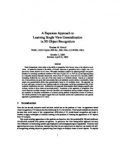
Figure 4: Toy graph

3

Experiments

We have designed a set of experiments to validate and evaluate our approach to norm detection. These experiments use either a toy graph with 6 nodes, illustrated in Figure 4, or a much larger random graph [Erdös and Rény, 1959] containing 35 nodes. We use the former to illustrate specific points about the technique, and the latter for empirical evaluation. Note that the large graph induces 1932 norm hypotheses and even the toy graph induces 100 possible norms. Table 2 summarises the parameters common to all experiments. For the experiments, we combine these graphs in a number of settings using either one or multiple norms in order to validate the ability of our approach to deal with multiple norms. Here, we differentiate the norms used to generate the observations, which we call Ng , from the norms inferred by our norm detection approach, which we call Nd . Since norm likelihood is estimated using log(odds) against there being no norm (rather than a probability), we infer the norms from a set of observations by ranking the odds of each norm (against no norm), and consider a fraction of the norms with the highest odds to be the norms in a society. We use this method of norm inference rather than, for example, a fixed numerical threshold, as the odds for a particular norm may be arbitrarily large, and unlike probabilities cannot be normalised to one. Thus, to translate the odds assigned to each hypothesis into an inference of which norms were detected, we rank the norms based on odds and pick a certain number of norms from the top. For example, consider the state of the norm odds illustrated in Table 3 after an agent following the model of Figure 2 observes a plan ha, b, ci. In this case, an agent can infer Nd = {never(e, d), · · · , eventually(e, c)} if it only wants to consider the norms with the highest odds. In the experiments, we ran an agent fully aware of the norms to generate a random set of observations following Table 3: Norm odds after observing ha, b, ci. Ranking 1 1 2 3

Norm Hypothesis never(e, d) .. . eventually(e, c) eventually(c, b) .. . next(c, e) .. .

Log(Odds) -1.90380897304 -1.90380897304 -2.59360606671 -2.99573227355



 weight(p)

X

pplanrec (o | n, g, P ) = pcomp 

P p∈non-viol-plans(plans(g,P ),n)

p0 ∈non-viol-plans(plans(g,P ),n)

 + (1 − pcomp ) 

X

= pcomp

weight(p) p(o | p) 0 p0 ∈plans(g,P ) weight(p ) X

weight(p)

p∈non-viol-plans(plans(g,P ),n) ∩ plans-containing(plans(g,P ),o)

X

p(o | p)

P

p∈plans(g,P )

X

weight(p0 ) 

weight(p)

p∈non-viol-plans(plans(g,P ),n)

+ (1 − pcomp )

weight(p)

p∈plans(g,P ) ∩ plans-containing(plans(g,P ),o)

X

weight(p)

p∈plans(g,P )

Figure 3: Likelihood of a path using plan recognition the algorithm of Figure 2 (i.e. random, but norm-compliant behaviour), while allowing for the possibility of occasional non-compliant behaviour with a probability set at 1% unless noted otherwise, thus (1 − pcomp ) = 0.01. We then applied our norm identification method to these observations in order to compute the odds of all possible norm hypotheses. Each experiment was repeated 50 times and averaged to smooth out any variations on the measurements due to the random nature of the observations. Our aim is to allow an agent to undertake norm-compliant behaviour, even without an exact model of the norms. One approach to doing this is to consider the T most likely norms, even if they are less likely than the null hypothesis (i.e. they may not exist since they are less likely than there being no norm). In such a situation, the agent can be thought of as acting conservatively, as it will avoid potentially permitted courses of action. Another approach is to have the agent consider only norms that are more likely than the null hypothesis. In the remainder of this work, we consider the functioning of an agent utilising norm identification and acting using the conservative approach, and evaluate its effectiveness in generating norm compliant behaviour. Our experiments measure precision and recall as a function of the number of observations supplied to the detection mechanism, we took these measures with and without a violation signal. Here, we measure recall in the usual way as the fraction of the Ng that are contained in the set Nd of detected norms. However, instead of measuring precision in terms of the ratio between the actual norms and the detected ones (Ng /Nd ), we measure precision in terms of the fraction of norm-compliant plan executions generated by an agent using a sample of the inferred norms to drive its behaviour. Given the number of norms that are indistinguishable from each other for a given a set of observations (e.g., in the possible plan executions of the graph of Figure 4, not next(c, e) is indistinguishable from never(c, e)), we argue that precision in the traditional sense is meaningless, whereas our notion captures the precision of ensuring norm-compliant behaviour. Specifically, we compute precision by updating the odds of each norm hypothesis after an observation and choosing the set Nd with the top T norms. We then randomly sample 35 norms from this set and use these 35 norms to generate 200 new plan executions according to the algorithm of Figure 2

counting the number of violations generated by monitoring for the norms in Ng . Finally, we compute precision as the ratio of plan executions with no violation within the sample. The results are illustrated in the graphs of Figure 5, which show that precision for inferring norms diminishes as the number of norms increases. In this experiment, we randomly selected elements of the power set P(Ng ) of the set of 7 norms in the scenario and, for each size of subset of P(Ng ), we determined precision and recall after 100 observations. We can see this effect by comparing the evolution of precision and recall in Figures 5a and 5b, where precision diminishes substantially when we change the number of active norms in an experiment from 2 to 7. This trend is easily seen in the graph of Figure 5c, which shows how precision and recall change as a function of the number of norms being used. We also evaluate the effect of a violation signal on the effectiveness of norm detection. The curves labelled with (V. Signal) in Figure 5 denote that the experiment now includes a violation signal, indicating to the norm detection mechanism that a sanction has just been applied. Here, the same experiments were repeated using the same graphs, but, where each violation occurs, a violation signal is added to the observation. The results show that, when there is a small number of norms (illustrated in Figure 5a), precision tends to remain the same, and recall is slightly worse over time. However, for a larger number of norms (illustrated in Figure 5b), precision and recall tend to increase slightly faster and remain so, as illustrated in the (V. Signal) curves in Figure 5c. This difference is more clearly visualised in the graphs of Figure 6, which compare precision and recall with and without violation signal under non-compliance rates of 0.01, 0.1 and 0.3. Here the ratio of precision and recall with a violation signal is often at least as good as without it (when violations do occur), and sometimes is 10% better as illustrated in Figure 6a, with an F1 that is almost always better with a violation signal, as illustrated in Figure 6b. The information gained from violation signals is even more pronounced when the number of violations increases, as we can see in the curves labelled with 10% or higher violations in Figure 6a, showing that, although precision only changes slightly (the norms, even when not precisely inferred, generate compliant behaviour), the recall ratio increases from an average of around 1.6 to around 1.8. This indicates that violation sig-

��

��

��

��

��

��

��

��

��

��

��

��

��

��

��

��

��

��

��

��

��

��

(a) Inferred norms (35 nodes, 2 norms)

��

��

��

��

��

��

��

��

��

��

(b) Inferred norms (35 nodes, 7 norms)

��

��

��

��

��

��

��

��

��

(c) Precision and recall as a function of norms

Figure 5: Inferred norms over time, with and without violation signals

4

��

��

��

��

��

��

(a) Ratio of precision and recall 1%-30% violations. ��

��

��

��

(b) Comparison of F1 score 1%-30% violations.

Figure 6: Comparison of Precision/Recall in experiments with and without violation signals (Viol = 1 − pcomp ).

nals allow a much more refined inference of the actual norms present in the system. The gap in F1 score shown in Figure 6b, likewise, widens substantially reflecting the improvements in norm detection in the presence of violation signals. In summary, our experiments show that our norm detection mechanism, when inferring norms based on a ratio of the highest computed odds results in significant precision and recall scores. Even in a graph with almost 2000 possible norms, our techniques enable an agent to generate norm-compliant plan executions between 70% and 99% of the time without any prior knowledge of the active norms within a system, achieving an F1 score between 0.6 and 0.95, as illustrated in Figure 6a and 6b. Our results also indicate a significant increase in effectiveness when a violation signal can be used, with a significantly better F1 score in such cases.

Discussion and Conclusions

We combine plan recognition (c.f., [Oren and Meneguzzi, 2013]), and a violation signal (c.f., [Savarimuthu et al., 2012; 2010]) to create a powerful new approach to norm identification. As our experiments indicate, we generate normcompliant behaviour in a norm-identifying agent at least 70% of the time in the presence of a large number of norms, and up to 99% for few norms. Importantly, we show that when norms are violated in an observable manner we substantially improve recall. As mentioned in Section 2, we assume that we can determine an agent’s starting point and goal. Considering AgentSpeak(L) style agents (and access to their plan libraries) then the identification of a plan, and from this its context and guard conditions, would allow an agent to determine the observed agent’s start point in many situations. Furthermore, once a plan has been identified, its goal can be trivially determined. While we assume that violation signals are observable, we do not assume that it is possible to associate specific norms with specific signals. We also assume that one cannot differentiate between sanction and punishment signals. Lifting such restrictions would simplify the problem, but is not realistic. We intend to pursue several avenues of future work. First, while our model permits it, we have not evaluated the effects of conflicting norms on the norm identification process or on the conservative strategy described in this paper, and we intend to investigate what additional mechanisms must be created to function in such domains. Given that many norms in our domain subsume others, we believe the use of a subsumption based norm conflict resolution mechanism [Vasconcelos et al., 2007] would result in an agent able to identify norms and act in a norm compliant manner in such environments. We also plan to investigate weighting mechanisms and their effects on norm identification. Such mechanisms could, for example, originate from trust information [Marsh, 1994]— highly trustworthy agents could be assumed to (normally) be norm compliant, while less trustworthy agents could be expected to generate more violation signals. Another source of weightings could originate from the plans themselves. In this work, we assumed that all plans to achieve some goal are equally likely to be used by an agent. However, some of these plans could be more expensive (e.g. from a resource utilisation point of view) than others, and a utility maximising agent would be expected to select cheaper plans (subject to normative constraints). We believe that the use of such weights would increase the rate at which norms are identified, and also increase the precision and recall of our approach.

References [Alrawagfeh et al., 2011] Wagdi Alrawagfeh, Edward Brown, and Manrique Mata-Montero. Norms of behaviour and their identification and verification in open multi-agent societies. International Journal of Agent Technologies and Systems (IJATS), 3(3):1–16, 2011. [Andrighetto et al., 2007] Giulia Andrighetto, Rosaria Conte, Paolo Turrini, and Mario Paolucci. Emergence in the loop: Simulating the two way dynamics of norm innovation. In Normative Multi-agent Systems, number 07122 in Dagstuhl Seminar Proceedings. Internationales Begegnungs- und Forschungszentrum für Informatik (IBFI), Schloss Dagstuhl, Germany, 2007. [Andrighetto et al., 2013] Giulia Andrighetto, Guido Governatori, Pablo Noriega, and Leendert W. N. van der Torre, editors. Normative Multi-Agent Systems, volume 4 of Dagstuhl Follow-Ups. Schloss Dagstuhl–Leibniz-Zentrum fuer Informatik, Dagstuhl, Germany, 2013. [Broersen et al., 2004] Jan Broersen, Frank Dignum, Virginia Dignum, , and John-Jules Ch. Meyer. Designing a deontic logic of deadlines. In Deontic Logic in Computer Science, volume 3065 of Lecture Notes in Computer Science, pages 43–56. Springer, 2004. [Erdös and Rény, 1959] P. Erdös and A. Rény. On random graphs. Publicationes Mathematicae, 6:290–297, 1959. [Luck et al., 2013] Michael Luck, Samhar Mahmoud, Felipe Meneguzzi, Martin Kollingbaum, Timothy J. Norman, Natalia Criado, and Moser Silva Fagundes. Normative agents. In Sascha Ossowski, editor, Agreement Technologies, volume 8 of Law, Governance and Technology Series, pages 209–220. Springer, 2013. [Mahmoud et al., 2012] Moamin A. Mahmoud, Mohd Sharifuddin Ahmad, Azhana Ahmad, Mohd Zaliman Mohd Yusoff, and Aida Mustapha. The semantics of norms mining in multi-agent systems. In Computational Collective Intelligence. Technologies and Applications, volume 7653 of Lecture Notes in Computer Science, pages 425–435. Springer Berlin Heidelberg, 2012. [Marsh, 1994] S. Marsh. Formalising trust as a computational concept. PhD thesis, University of Stirling, 1994. [Oren and Meneguzzi, 2013] Nir Oren and Felipe Meneguzzi. Norm identification through plan recognition. In 15th International Workshop on Coordination, Organizations, Institutions, and Norms, pages 161–175, 2013. [Savarimuthu et al., 2010] Bastin Tony Roy Savarimuthu, Stephen Cranefield, Maryam A. Purvis, and Martin K. Purvis. Obligation norm identification in agent societies. Journal of Artificial Societies and Social Simulation, 13(4):3, 2010. [Savarimuthu et al., 2012] Bastin Tony Roy Savarimuthu, Stephen Cranefield, Maryam A. Purvis, and Martin K. Purvis. Identifying prohibition norms in agent societies. Artificial Intelligence and Law, pages 1–46, 2012. [Serban and Minsky, 2009] Constantin Serban and Naftaly H. Minsky. In vivo evolution of policies that govern a distributed system. In POLICY 2009, IEEE International Symposium on Policies for Distributed Systems and

Networks, London, UK, 20-22 July 2009, pages 134–141, 2009. [Vasconcelos et al., 2007] Wamberto W Vasconcelos, Martin J Kollingbaum, and Timothy J Norman. Resolving conflict and inconsistency in norm-regulated virtual organizations. In Proceedings of the Sixth International Conference on Autonomous Agents and Multiagent Systems (AAMAS 2007), pages 632–639, Honolulu, Hawaii, USA, 2007.