introduction to Fluid Dynamics, so a student interested in pursuing any of the
ideas further should consult any of the many excellent text books that exist in this
...
A BRIEF INTRODUCTION TO FLUID DYNAMICS M.G. Worster University of Cambridge
Contents
Preface A brief introduction to fluid dynamics
v
page vii 1
Preface
This book is an account of lectures that I gave at AIMS (the African Institute of Mathematical Sciences) in 2008. It is not a text book in the conventional sense, neither is it a set of lecture notes that I lectured from, still less lecture notes that I lectured to, given to students in advance. Rather it is a diary, summarizing and reflecting upon what I had tried to convey to the students in the hour or two immediately preceding writing it and including the various exercises and assignments given to the students to help them get to grips with the ideas. It reflects the fact that lectures at AIMS are dynamic, interactive sessions: to be sure, there is some didactic delivery of material but that is interspersed with problem-solving activities and many, many questions so that the educational process is much more of a conversation than is typical of most university courses. Some of that conversational style has carried over into the writing. Where, in the course of writing, I discovered some small point that I had omitted to mention or some additional clarification or illustration that I felt would vii
be helpful I allowed myself to include it and then brought it to the students’ attention the following day. Other than that, I have made no attempt to provide a comprehensive introduction to Fluid Dynamics, so a student interested in pursuing any of the ideas further should consult any of the many excellent text books that exist in this subject. The first two times that I lectured at AIMS, I shared the three-week course with another lecturer: Daya Reddy from the University of Cape Town in 2004 and Keith Moffatt from Cambridge University in 2006. I nevertheless wanted my half course to be complete in itself and to convey something meaningful about Fluid Dynamics as an important topic of current research to students who had never met the subject before. I felt it important that the students learn about real, viscous fluids, to have a taste of analytical, numerical and experimental approaches to understanding and quantifying the flow of fluids, and to experience the satisfaction and some of the limitations of making theoretical predictions of experimental flows. I am extremely grateful to the students who prepared the figures and tables: Khumbo Kumwenda; Doreen Mbabazi; Mercy Njima.
viii
A brief introduction to fluid dynamics
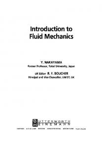
Viscous fluids All ordinary fluids resist motion because of their viscosity. Our common experience tells us that fluids like water and air are less viscous than oil and syrup but we need a way to quantify that experience. Students at AIMS began by dropping steel ball bearings of different diameters into golden syrup contained in a measuring cylinder (see figure 1). They measured the distance travelled by each ball as a function of time and produced the results shown in table 1. Their visual experience, confirmed by the data, was that each ball fell at a constant speed. Therefore the forces on the sphere must be in equilibrium. What are they?
Forces on a body moving through a fluid The reason the ball falls is because gravity acts on it. The gravitational force on the ball is its weight = ρs V g, 1
2
A brief introduction to fluid dynamics time,t/s
distance /cm
distance /cm
distance /cm
distance /cm
0 5 10 15 20 25 30 35 40 45 50 55 60
0 0.5 0.9 1.5 2.0 2.4 2.9 3.4 3.8 4.4 4.8 5.2 5.6
0 0.8 2.4 3.5 4.5 5.6 6.5 7.5 8.5 9.5 10.9 11.9
0 0.5 1.5 4.5 6.4 8.4 10.4 12.4 14.3 16.2 18.0 19.7
0 3.2 6.1 8.9 11.8 14.2 16.7 19.2
Table 1. Data collected of the distance travelled by steel ball bearings of different diameters, d falling through golden syrup. The different diameters are: d = 3.96 mm, d = 6.34 mm, d = 9.52 mm, d = 12.68 mm respectively.
where ρs is the density of the (steel) ball, V is the volume of the ball and g is the acceleration due to gravity. However, we also know that a body submerged in a fluid experiences a buoyancy force: corks rise upwards in water and a helium-filled balloon rises upwards in air. That buoyancy force is also called the upthrust = ρf V g, where ρf is the density of the fluid. This relationship, known as Archimedes principle, says that the upthrust on a body submerged in a fluid is equal to the weight of the fluid displaced by the body. We can derive this result as follows. If the body moves downwards a distance z, as shown in
A brief introduction to fluid dynamics
3
figure 2, then the change in potential energy of the system is φ = −(ρs V )gz + (ρf V )gz : the body loses potential energy but the fluid that is displaced in order to make way for the body and fill the gap left behind gains potential energy. The net downwards force on the body is therefore dφ = ρs V g − ρf V g = weight − upthrust. dz If the densities of the body and the fluid are different then there is a net gravitational force (weight−upthrust) on the body, which would cause it to accelerate if there were no other forces acting. The additional force that allowed the ball bearing to fall at constant speed is the viscous shear stress. F =−
Normal stress Stress is force per unit area. It is a vector quantity (it has direction as well as magnitude) and the stress exerted by a fluid on a surface can be considered in two parts. We are used to the idea of the force per unit area exerted by a liquid or a gas on a stationary object being the pressure. Pressure p is part of the normal stress exerted by a fluid on the surface of a body, the component of the stress that acts normal to the surface. If there is no fluid motion then the stress is given entirely by τ = −pn, with the convention that the normal vector n points into the fluid.
4
A brief introduction to fluid dynamics The no-slip condition
It is an experimental fact that, except possibly on molecular scales at which the fluid can no longer be considered a continuum, the fluid in contact with a moving solid body has the same velocity as the body. This is known as the noslip condition: the fluid does not slip tangentially relative to the surface of the body.
Tangential viscous shear stress In consequence of the no-slip condition, it is not difficult to imagine, as illustrated in figure 3, that when a body moves through a fluid that was stationary there is a gradient in the velocity field of the fluid: the fluid is in motion near the body and at rest far from the body. Gradients in fluid velocity are called shear and it is the shear of a fluid, the relative motion of bits of fluid near to one another, that causes dissipation of kinetic energy, experienced by the body as a drag. The shear stress exerted by the fluid on the body is a force per unit area acting tangentially to the surface of the body. It is proportional to the shear in the fluid adjacent to the surface. We shall quantify these statements a little in the next lecture.
A viscous gravity current Our next experience of fluid flow comes from watching a puddle of spilt syrup spreading over a horizontal plane, as shown in figure 4. Students released about 190 ml of the syrup from a cylinder and measured the radius of the resulting puddle as a function of time. Their measurements
A brief introduction to fluid dynamics
5
are reproduced in table 2. We can think about what controls the flow of syrup in this experiment in terms of the forces acting on it. Time, t/s
rN1 /cm
rN2 /cm
rN3 /cm
rN4 /cm
2
5
5
5
5
4
6
6
6
6
6
7
7
7
7
8
7.5
7.5
7.5
7.5
10
8
8
8
8
15
8.1
8.1
8.1
8.5
30
8.5
8.5
9
9
45
9.2
9.2
9.2
9.5
60
9.5
9.6
9.8
9.8
90
10
10
10
10.3
120
10.1
10.2
10.5
10.5
Table 2. Data collected of the measurements of the radius of the resulting puddle as a function of time.
The current is thicker in the middle and thins at larger radii. Therefore, there is a higher pressure in the syrup near the middle and a lower pressure towards the edges. The horizontal pressure gradient provides the driving force for the flow. However, the fluid does not accelerate. In fact, it was observed to slow down with time. There is an opposing viscous shear stress exerted on the fluid by the horizontal plane in consequence of the shear generated as
6
A brief introduction to fluid dynamics
the fluid above the plane flows horizontally while the fluid adjacent to the plane is stationary because of the no-slip condition. Our aim in the next few lectures is to understand enough about viscous shear stresses and how to express mathematically the physical principles we have discussed in this lecture to be able to predict the flow of a viscous gravity current.
Assignment The first exercises relate to the measurement of viscosity made by dropping ball bearings through a viscous fluid. (i) For each of the experimental runs, plot the distance travelled by the ball as a function of time. (ii) Use your graphs to determine the speed of the ball in each case. What do you notice? (iii) Given that the force on a sphere of radius a moving at speed U through a viscous fluid is F = 6πµaU , determine the dynamic viscosity µ of the fluid. (You will need to find the densities of steel and of golden syrup. E.g. use the internet.) Do you get the same value of µ in each experiment? Explain what you find. The following exercises relate to the experiment with a viscous gravity current, for which data was collected of the radius of the current rN at various times t. Four measurements of rN were made at each time.
A brief introduction to fluid dynamics
7
(iv) Plot a graph of r against t. You could plot each value of r separately (on the same graph) and the average of the rN ’s at each time. (v) Supposing that rN = atb , determine the constants a and b from the data.
Dynamic viscosity Consider a layer of fluid between two parallel rigid plates separated by a distance h, as shown in figure 5. The lower plate is held stationary while the upper plate is forced to move horizontally at a fixed speed U . It is found experimentally that the force per unit area that must be exerted on the upper plate is proportional to U and inversely proportional to h: U force ∝ . area h Since the plate moves with constant velocity, the forces on it must balance and so the force per unit area exerted by the fluid on the plate is U . h The tangential viscous shear stress τs is in the opposite direction to the motion of the plate. The constant of proportionality µ is called the dynamic viscosity of the fluid. τs = −µ
Tangential shear stress The no-slip condition implies that the velocity of the fluid between the parallel plates must vary between zero at the
8
A brief introduction to fluid dynamics
lower plate to U at the upper plate. The experimental observations stated above require that the variation be linear and that the term U/h is therefore equal to the gradient of the fluid velocity. In general, the tangential shear stress exerted by a fluid on a rigid surface is τs = µ
∂u = µn · ∇u, ∂n
where u is the component of the velocity field tangential to the surface and n is the normal to the surface pointing into the fluid.
Parallel shear flow Consider a fluid flow of the form u = (u(y), 0, 0) in Cartesian coordinates (x, y, z) and the forces acting on a slab of fluid parallel to the x axis. The vertical sides of the slab experience pressure forces in the x direction, while the horizontal sides of the slab experience tangential shear stresses in the x direction from the surrounding fluid, as depicted in figure 6. Since the flow is steady, the forces on the slab must balance, giving us p(x)δy − p(x + δx)δy + τs (y + δy)δx + τs (y)δx = 0. Noting that the normal to the upper surface of the slab pointing into the surrounding fluid is in the positive y direction, while the normal to the lower surface of the slab pointing into the surrounding fluid is in the negative y direction, we see that τs (y + δy) = µ
∂u (y + δy) ∂y
while
τs (y) = −µ
∂u (y). ∂y
A brief introduction to fluid dynamics
9
Therefore, if we divide our expression by δxδy, we obtain ∂u µ ∂u ∂y (y + δy) − µ ∂y (y)
δy
−
p(x + δx) − p(x) = 0. δx
Taking the limits δx → 0, δy → 0, we obtain finally µ
∂2u ∂p = . ∂y 2 ∂x
Resolving forces in the y direction (transverse to the flow) using a similar approach gives us 0=
∂p . ∂y
Extensions (left as exercises for the student) If the flow is unsteady and there is a body force (force per unit volume) f = (fx , fy , 0) then ρ
∂u ∂t
= mu
0
= −
∂ 2 u ∂p − + fx , ∂y 2 ∂x
∂p + fy ∂y
For example, if x points vertically downwards then f = ρg.
Boundary conditions At a stationary, rigid boundary the velocity is zero in consequence of the no-slip condition: u =
0
at a stationary, rigid boundary
or u =
U
at a rigid boundary moving with speed U .
10
A brief introduction to fluid dynamics
At a fluid–fluid boundary the velocity and both components of the stress are continuous. For parallel viscous flow this implies that the pressure and the tangential viscous stress are both continuous: � � ∂u =0 at a fluid–fluid boundary, [p] = 0, µ ∂n where [ ] denotes the jump in the enclosed quantity across the boundary. In many cases, one of the fluids is much less viscous than the other and exerts negligible stress on the flow of interest, in which case we approximate the boundary as being stress-free and use the conditions [p] = 0,
∂u =0 ∂n
at a stress-free boundary.
Parallel flow in a channel As a first example, we can use these equations to determine the parallel flow of fluid in a channel between two parallel, rigid walls a distance h apart, as shown in figure 7. The flow is driven by a pressure difference between the ends of the channel. If the flow is steady and the channel is horizontal, our two equations become 0=µ
∂ 2 u ∂p − , ∂y 2 ∂x
0=−
∂p − ρg. ∂y
The second equation is readily integrated to show that the pressure p = −ρgy + C(x), where C(x) is an arbitrary function of x only. The first term on the right-hand side is simply the hydrostatic pressure,
A brief introduction to fluid dynamics
11
which does not cause any flow. From this equation, we see that ∂p/∂x = C ′ (x) is at most a function of x. But, since u(y) is a function of y only, the first equation shows that in fact ∂p/∂x is constant, which we denote by −G. Our problem thus reduces to solving µ
∂2u = −G ∂y 2
in 0 < y < h
with boundary conditions u(0) = u(h) = 0 in consequence of the no-slip condition. This equation and boundary conditions are readily integrated to give u=
G y(h − y). 2µ
We see that the velocity profile is parabolic. This flow is known as 2-D Poiseuille flow. Now that we have a mathematical expression, we can determine certain properties of the flow. For example, the shear stresses at the lower and upper boundaries are ∂u Gh Gh ∂u , τs (h) = −µ . = = τs (0) = µ ∂y y=0 2 ∂y y=h 2
If the channel has length L then the total viscous force exerted by the fluid on the walls per unit width in the z direction is [τs (0) + τs (h)]L = GL h = ∆p h, which is equal to the difference in the pressure forces acting at the ends of the channel. We can also determine the volume flux (volume of fluid
12
A brief introduction to fluid dynamics
passing any cross section of the channel per unit time) per unit width in the z direction Z h Gh3 . q= u(y) dy = 12µ 0 Note that the volume flux is proportional to h3 : a channel twice as deep will transport eight times as much fluid per unit time for a given pressure gradient driving the flow. Students should now try question (1) in the following exercises before looking at the outline solution that follows.
Poiseuille flow in a pipe Consider the parallel flow u(r) of viscous fluid in a circular pipe of radius a, depicted in figure 8. The longitudinal forces on a cylinder of fluid of radius r < a and length δx consist of viscous shear stresses on the curved surface and pressure forces on the ends. In steady flow, there is no net force on this fluid cylinder and so � � ∂u + πr2 [p(x) − p(x + δx)] = 0 2πrδx µ ∂r which gives, in the limit δx → 0,
∂u 1 ∂p = r. ∂r 2µ ∂x
Once again, it can be shown that ∂p/∂x = −G is constant. We can therefore integrate the equation with suitable boundary conditions (question 2 in the exercises) to show that G 2 (a − r2 ). u= 4µ
A brief introduction to fluid dynamics
13
Note that the volume flux Z a πGa4 q= 2πru dr = 8µ 0 is proportional to the fourth power of the radius: a pipe twice as wide will transport sixteen times as much fluid per unit time for a given pressure gradient driving the flow! We shall revisit this flow once we have a general vector equation for three-dimensional fluid flows, when the assumptions made here can be made more rigorous.
Exercises (i) Consider the steady flow of a layer of fluid of uniform thickness h down a rigid vertical plane. Assume that the surrounding air exerts no stress on the fluid. (a) Draw a picture of this situation including a rough sketch of the velocity profile of the fluid. (b) Write down the dynamical equation governing the vertical velocity of the fluid. (c) What boundary conditions should be applied to this flow? (d) Calculate the velocity profile and from that the mass flow rate (per unit width) of fluid down the plane. (ii) Compute the velocity profile and volume flux for Poiseuille flow of a fluid of dynamic viscosity µ in a circular pipe of internal radius a subjected to a pressure gradient −G along the pipe. (iii) Two immiscible layers of fluid flow steadily down a plane inclined at an anlge θ to the horizontal. The
14
A brief introduction to fluid dynamics lower layer, in contact with the plane, has density ρ, dynamic viscosity µ and uniform depth h normal to the plane. The upper layer, on top of the first, has the same density ρ but dynamic viscosity βµ and depth αh. Using coordinates x along the plane and y perpendicular to it, write down the equation of motion and the boundary conditions at the plane and the free top surface. What are the boundary conditions that apply at the interface between the two fluids? Find the velocity field in each layer on the assumption that it depends only on y. Why does the velocity profile in the bottom layer depend on α but not on β?
Solution to question 1 A sketch of the flow is given in figure 9. Note that I have chosen a coordinate system in which x points in the direction of the flow, which in this case is downwards, and y points across the flow. The equation of motion in the y direction gives ∂p =0 ∂y
⇒
p = p(x)
only.
But pressure is continuous across a fluid–fluid boundary, so the pressure is just equal to the atmospheric pressure patm , which we can assume to be constant on the scale of the flow. Therefore the equation of motion in the x direction reduces to ∂2u 0 = µ 2 + ρg. ∂y
A brief introduction to fluid dynamics
15
The velocity u(y) is subject to no slip at the solid boundary and no stress at its boundary with the air: ∂u (h) = 0. ∂y
u(0) = 0,
It is now straightforward to integrate the differential equation and apply the boundary conditions to obtain u=
ρg y(2h − y). 2µ
From this we can calculate the surface velocity u(h) =
gh2 2ν
and the volume flux q=
gh3 , 3ν
where we have introduced the kinematic viscosity ν = µ/ρ.
Couette versus Poiseuille Consider the problem of wind blowing over a large lake, exerting a constant stress S on the surface, as depicted in figure 10. What is the steady flow established in the lake after a long time? Let’s assume that the lake has a a constant depth h0 before the wind blows. The wind will tend to push water towards the downwind end of the lake and thus establish a small variation in depth h(x). If we also assume that the flow in the lake in parallel (except near
16
A brief introduction to fluid dynamics !"#$%&'()*+,-./0123456789:;?@ABCDEFGHIJKLMNOPQRSTUVWXYZ[\]^_`abcdefghijklmnopqrstuvwxyz{|}~
air
fluid y
patm
x
g
y=0
y=h
Fig. 0.1. Figure 9. A film of viscous fluid of thickness h flowing down a vertical, rigid wall at y = 0.
the ends) then µ
∂ 2 u ∂p − ∂y 2 ∂x
=
0,
∂p − ρg ∂y
=
0.
−
The second equation can be integrated once to give p = −ρgy + ρgh(x) + patm , given that the pressure is equal to atmospheric pressure at the surface of the lake. This expression can be used in the
A brief introduction to fluid dynamics
17
Fig. 0.2. Figure 10. A wind blowing over a long, shallow lake exerts a constant stress S on the surface of the lake. The pressure built up as water collects at the down-wind end of the lake drives a return flow near the bottom of the lake.
first equation to give µ
∂2u = ρghx , ∂y 2
where hx ≡ ∂h/∂x. This equation is subject to the boundary conditions u(0) = 0,
µ
∂u (h) = S ∂y
reflecting no slip at the bed of the lake and the imposed stress at the surface. It is now a straightforward exercise to determine that S ghx y(2h − y) + y. u=− 2ν µ The first term on the right-hand side is driven by the pressure gradient arising from the (small) slope of the lake. Parallel flows driven by longitudinal pressure gradients are generally classed as Poiseuille flows and are parabolic in
18
A brief introduction to fluid dynamics
profile. The second term on the right-hand side is driven by the surface stress. Such flows are classed as Couette flows and are linear in profile. It is a good exercise to make rough sketches of the flow profile for different cases, for example when either S or hx is zero or for different signs of hx for a given, positive S. A little playing will show you that when S is non-zero it is possible to have a positive surface flow with a negative return flow at depth if hx is sufficiently large. If there is a steady state of the whole system then the volume flux across any vertical cross section must be zero, else the water will build up on one side of the cross section and diminish on the other. The volume flux (per unit width of the lake) is
q=
Z
0
h
u dy = −
Sh2 gh3 hx + , 3ν 2µ
which is zero if hx =
3S . 2ρgh
At a wind speed of 10 m s−1 the wind stress S is about 10−6 atm (about 10−1 N m−2 ) whereas the pressure ρgh at the bottom of a 10 m lake is about 1 atm (about 105 N m−2 ), so hx is about 10−6 : the difference in depth of the lake would be a mere millimetre across a lake of horizontal dimensions of 1 km and the approximation we made that h is almost constant is an extremely good one!
A brief introduction to fluid dynamics
19
Unsteady parallel viscous flows In the example above we considered the steady flow that was established once the wind had been blowing steadily for a long time. But we can also find out how the flow develops from rest after the wind starts to blow. We’ll actually consider a slightly simpler problem. Rather than forcing the flow with a constant stress, let us imagine that the horizontal lower boundary y = 0 of a semi-infinite fluid region is set into motion at a constant horizontal speed U , as shown in figure 11. Assume that the fluid flows parallel to the boundary and that there is no variation of the system in the horizontal direction x. The parallel flow equation in the x direction therefore reduces to ∂2u ∂u = ν 2. ∂t ∂y This is a partial differential equation with two space derivatives and one time derivative. Therefore we need two boundary conditions and one initial condition. The boundary conditions are the no-slip condition at the moving boundary and that far from the boundary the fluid is at rest: u=U
at y = 0;
u → 0 as
y → ∞.
The initial condition is that the fluid not in contact with the boundary is at rest: u = 0 at t = 0 for
y > 0.
There are many mathematical techniques that can be used to solve this linear partial differential system. We shall tackle it using scaling analysis and similarity theory.
20
A brief introduction to fluid dynamics Similarity solution
Notice first that the equation is linear and forced only by the boundary condition at y = 0. This immediately tells us that u = U f (y, t), where f is a dimensionless function. A mathematical function, such as f , must have dimensionless arguments, whereas the independent variables y and t have dimensions of length and time respectively. We might measure length in metres or feet and time in seconds or years but the mathematical function must be independent of such a choice. Therefore, we must find or choose characteristic length and time scales L and T and write instead � � y t . , u = Uf L T If we substitute this expression into the differential equation we can see that f is a function of dimensionless variables only if √ U U ⇒ L ∝ νT . ∝ν 2 T L There is no other dimensional information in the system of equation and boundary conditions that relates to L or T , so the only characteristic time scale in the problem is√the elapsed time t itself. We therefore set T = t and L = νt (choosing the constant of proportionality to be one) and write � � y u = Uf √ , 1 . νt
A brief introduction to fluid dynamics
21
This shows that in fact f depends only on the combined variable y η= √ , νt the so-called similarity variable, rather than on y and t independently, and we can write u = U h(η). It is a straightforward exercise to substitute this expression into the partial differential equation and determine that h satisfies the ordinary differential equation − 21 ηh′ = h′′ and that the two boundary conditions and one initial condition reduce to the two conditions h(0) = 1,
h → 0 as
η → ∞.
The linear, separable, first-order equation for h′ can be integrated to give h′ = Ae−η
2
/4
,
where A is a constant of integration. This can be further integrated to give Z η Z η/2 2 2 h=A e−ξ /4 dξ + B = 2A e−s ds + B, 0
0
using a simple change of variables ξ = 2s. The integral in this expression cannot be evaluated with simple functions but can be expressed in terms of the error function Z z 2 2 e−s ds, erf z ≡ √ π 0
22
A brief introduction to fluid dynamics
which is sketched in figure 12a. The error function has the properties that erf (0) = 0, erf z → 1 as z → ∞ and it is odd. The boundary conditions on h can now be applied to show that h(η) = 1 − erf (η/2) ≡ erfc (η/2) , in terms of the error function complement erfc (z) = 1 − erf (z), sketched in figure 12b. Piecing this all together, we find that � � y √ . u(y, t) = U erfc 2 νt The velocity profile is sketched at one particular time in figure 11. We see that it is a decaying function √ of y, with a characteristic decay length proportional to νt. The profiles at different times are self-similar in that they have the same mathematical form at all times with the distance variable simply scaled with a time-dependent characteristic length scale.
Viscous boundary layers The flow just found is an example of a viscous boundary layer: the shear is confined to a narrow region close to the solid boundary of the fluid. In the case just studied, the thickness of the boundary layer grows with time but in many cases the boundary layer can be confined to a small region. For example, if the solid plate in the previous example were finite rather than infinite then the boundary layer stops growing roughly when information about the leading edge of the plate reaches the point in question. Such information reaches a distance x from the leading edge in a time
A brief introduction to fluid dynamics
23
t roughly equal to x/U . At that time the growing viscous boundary layer will have reached a characteristic thickness p √ of νt = νx/U , as shown in figure 13. An estimate of this thickness for an aeroplane wing with a width of say 1 m, flying at 100 m s−1 in air, which has kinematic viscosity of approximately 10−6 m2 s−1 , is approximately 10−4 m or about 0.1 mm. Outside of this extremely thin boundary layer the fluid velocity is equal to the free-stream velocity: the no-slip condition is not apparent on the large scale!
Exercise A further example illustrating the confinement of shear to the region of fluid close to a rigid boundary is given by the case of a semi-infinite fluid whose rigid lower boundary is oscillating in its own plane with velocity U = U0 cos ωt. By writing the velocity parallel to the boundary as u(y, t) = Re[U0 f (y)eiωt ], determine the velocity field. In particular, show that, as the distance y from the plane increases, the amplitude of p fluid motion decays within a characteristic distance of ν/ω, as shown in figure 14. Calculate the mean power that must be supplied per unit area of the boundary in order to sustain its motion.
Viscous gravity currents We are now in a position to calculate the flow of syrup poured onto a horizontal surface that was measured in our second experiment. This is a significant problem that brings together all the ideas we have met so far. We’ll start by con-
24
A brief introduction to fluid dynamics
sidering a two-dimensional version of the problem, as shown in figure 15. We’ll assume that because the current is long and thin the flow is almost parallel, u = (u(y, t), 0), and use the equations of parallel flow ρ
∂ 2 u ∂p − , ∂y 2 ∂x
∂u ∂t
= µ
0
= −
∂p − ρg. ∂y
We start by estimating the sizes of the terms in the first of these equations. Suppose that the characteristic scale for variations in the x direction is L and in the y direction is H, that the characteristic velocity scale is U and that therefore the characteristic time scale T = L/U . The ratio of the inertial term on the left-hand side of the first equation to the first term on the right-hand side, representing viscous stresses, is U H2 U U : 1. ρ :µ 2 = T H νL Therefore, from a formal (asymptotic) point of view, the inertial term can be neglected relative to the viscous term if U H 2 /νL ≪ 1. From a practical point of view, we can estimate that the velocities in our experiment were never more than about 10 cm s−1 , the thickness was about 1 cm and the length about 10 cm. The dynamic viscosity of golden syrup at 20◦ C is about 500 cm2 s−1 . These estimates give U H 2 /νL ≈ 2 × 10⁻³ at most, so it is a very good approximation to neglect inertia in our analysis of the experiment. Integrating the momentum equation in the y direction, we find that the pressure p = −ρgy + ρgh(x, t) + patm ,
A brief introduction to fluid dynamics
25
noting that the pressure is equal to the atmospheric pressure patm at the top surface of the current y = h. The momentum equation in the x direction and the associated boundary conditions are then µ
∂2u ∂y 2
µ
= ρg
∂h , ∂x
u
= 0
at y = 0,
∂u ∂y
= 0
at y = h.
Just as in the problem we looked at of a wind stress driving flow in a lake, the elevation h(x, t) of the free surface is determined by a constraint on the volume flux. In the present case we have the constraint that the total volume of fluid is fixed: Z xN h(x, t) dx = V (const.) 0
Scaling analysis We can deduce a lot about the solution of this problem simply from scaling the governing equations. The balance of terms in the momentum equation gives µ
U H ∼ ρg , h2 L
while the volume constraint shows that HL ∼ V.
26
A brief introduction to fluid dynamics
It is a simple exercise to combine these two expressions to show that � 3 �1/5 gV L∼ T . ν There are no further constraints on these scales, so we have no choice but to scale time with the elapsed time t. This gives us a similarity solution, as we shall see in detail below. For the moment, we can deduce that xN = ηN
�
gV 3 t ν
�1/5
,
where ηN is a constant of proportionality that has yet to be determined. However, without solving the governing differential equations, we have managed to deduce that the length of the current is proportional to the one-fifth power of time and also how the rate of spreading depends on the volume V of the current, its viscosity ν and the gravitational acceleration g. We can also determine that the thickness of the current scales as � 2 �1/5 νV . H∼ gt Velocity profile and volume flux The first step towards a complete solution is to integrate the momentum equation and apply the boundary conditions to obtain g ∂h u=− y(2h − y) 2ν ∂x
A brief introduction to fluid dynamics
27
and compute the volume flux (per unit width) Z h gh3 ∂h h dy = − q= . 3ν ∂x 0 Conservation of mass Consider the fluid crossing two nearby vertical sections at positions x and x + δx, as shown in figure 16. If there is more fluid entering this region than leaving it then the elevation of the free surface must increase. Conservation of mass in this region shows us that [q(x) − q(x + δx)] δt = δhδx. Dividing this expression by δxδt and taking the limits δx → 0, δt → 0, we obtain ∂h ∂q + = 0. ∂t ∂x This is a general continuity equation expressing mass conservation in one dimension. In the particular case we are considering, we can use the expression for the mass flux q obtained above to write � � ∂ gh3 ∂h ∂h . = ∂t ∂x 3ν ∂x Similarity solution The equation for h(x, t) that we have just derived is a nonlinear partial differential (diffusion) equation. Usually, it will require numerical solution, there being no general analytical method to solve it. However, our scaling analysis
28
A brief introduction to fluid dynamics
has told us that there is a similarity solution in which � 2 �1/5 � 3 �−1/5 νV x gV h= t f (η) where η = = x gt L ν and f is a dimensionless function of the dimensionless similarity variable η. We can use these expressions in the partial differential equation for h to find the ordinary differential equation 1 5f
+ 51 ηf ′ + 31 (f 3 f ′ )′ = 0
for the scaled thickness f of the current. This equation can be integrated once to give 1 5 ηf
+ 31 f 3 f ′ = 0
by choosing the constant of integration so that the flux q ∝ f 3 f ′ = 0 at η = 0. One further integration and application of the boundary condition f = 0 at η = ηN gives �1/3 � 2 9 1/3 . ηN − η2 f = 10 Finally, the global volume constraint in scaled form is Z ηN f (η) dη = 1. 0
Substituting the expression for f (η) into this integral and making the change of variables η = ηN z, we obtain the equation Z 1 � 9 1/3 5/3 η (1 − z 2 )1/3 dz = 1. N 10 0
The integral in this expression can be written in terms of the Beta function or Gamma functions as Z 1 Γ( 1 )Γ( 4 ) (1 − z 2 )1/3 dz = 12 B( 12 , 43 ) = 2 11 3 , 2Γ( 6 ) 0
A brief introduction to fluid dynamics
29
which gives us ηN =
"�
9 10
#−3/5 �1/3 √ π Γ( 13 ) ≈ 1 · 13. 5 Γ( 56 )
The horizontal extent of the current is therefore given by � 3 �1/5 gV xN ≈ 1.13 t . ν Remarkably, most of this expression was found by scaling analysis: only determination of the multiplicative constant (almost unity) required the solution of differential equations.
30
A brief introduction to fluid dynamics Assignment
In class we solved the similarity equations for a two-dimensional gravity current analytically. As an illustration of one method for solving nonlinear ordinary differential equations numerically, we shall solve the same equations using a computer. We will build up a code in stages. It is possible to find ready-made packages to do everything below but we will learn a lot on the way if we write the code ourselves. The first step (sections 1 & 2) is to solve a first-order differential equation numerically. We will explore two methods: a Simple Euler method and a two-step Runge Kutta method. In each case, we will use our programme to compute the solution of the differential equation dy = −y dx with y = 1 at x = 0. It is useful to think in terms of a general problem dy = f (x, y) dx y = y0
at x = x0 .
1. Euler Method In this method, we compute the derivative at a point (xN , yN ) and use this derivative to advance along the tangent line by an increment ∆x. Thus yN +1 := yN + fN ∆x,
(1)
A brief introduction to fluid dynamics
31
where fN = f (xN , yN ). We can use (1) repeatedly, starting from the known initial values x0 and y0 . Write a code to solve a first-order differential equation with the Euler method and use it to solve the example above. (i) Use ∆x = 0.2 and integrate from x = 0 to x = 2. Plot the data points (xN , yN ) on a graph of y = e−x . What do you notice? (ii) Use your programme to compute y(2) for different values of ∆x. Examine the behaviour of |y(2) − e−2| as ∆x is succesively halved.
2. Two-step method RK2 In this method, we compute the derivative at a point (xN , yN ) and use this derivative to advance along the tangent line by half an increment ∆x/2. Thus yN +1/2 := yN + fN ∆x/2.
(2a)
We then compute the derivate fN +1/2 = f (xN +1/2 , yN +1/2 ) at this half-way point and use that derivative to step along the whole increment. Thus yN +1 := yN + fN +1/2 ∆x.
(2a)
Write a code to solve a first-order differential equation with the two-step method and use it to solve the example above. (i) Use ∆x = 0.2 and integrate from x = 0 to x = 2. Plot the data points (xN , yN ) on top of a graph of y = e−x . What do you notice?
32
A brief introduction to fluid dynamics
(ii) Use your programme to compute y(2) for different values of ∆x. Examine the behaviour of |y(2) − e−2| as ∆x is succesively halved. (iii) In each case (a) and (b), contrast your results with those you obtained in section 2.
3. Shooting We shall look at solving a second-order differential equation with boundary conditions applied at each end of a domain. The example we shall use is d2 y + y = −e2x dx2 with
and
y
=
0 at x = 0,
y
=
0 at x = 1.
We solve this as a system of first-order equations by writing y1
=
y,
y2
=
dy . dx
Then dy1 dx dy2 dx
=
f1 (x, y1 , y2 ) ≡ y2 ,
=
f2 (x, y1 , y2 ) ≡ −e2x − y1 .
The difficulty is that our integration method (Euler or Two-Step) starts from one end and steps towards the other.
A brief introduction to fluid dynamics
33
It therefore needs boundary conditions for both of y1 and y2 at the same end. We get around this by starting at x = 0, for example, using the boundary condition that we know there, namely y1 = 0, and guessing a value for y2 . We then integrate (shoot) equations (3a) and (3b) until x = 1 and see how close we are to (the target) y1 (1) = 0. Modify your programme for the two-step method to integrate equations (3a) and (3b) from x = 0 to x = 1, starting with y1
=
0,
y2
=
p,
where p is a parameter (your guess) that can be varied. Allow your programme to accept p as an input, and for each value of p that you guess plot a graph of y1 (x). Look at how the graph changes as p changes. Can you guess a value of p to three significant figures that causes y1 (1) = 0?
4. Gravity current The equations governing the self-similar shape f (η) of a two-dimensional gravity current are 1 5f
+ 51 ηf ′ + 13 (f 3 f ′ )′ Z
=
0
f (ηN ) =
0
ηN
f (η) dη
=
1,
0
where the end of the current ηN has also to be determined. It is convenient to implement the volume constraint (4c)
34
A brief introduction to fluid dynamics
by writing g(η) =
Z
η
f (ξ) dξ,
0
so that we have an additional differential equation g′ = f with g(0) = 0
and
g(ηN ) = 1.
It is also convenient to map the domain of the problem onto [0, 1] by writing x=
ηN − η . ηN
[Note that η = ηN corresponds to x = 0.] The system of equations to be solved is then � 3 � 2 2 2 5f fx + ηN (f − (1 − x)fx ) , 3 5f
fxx
=
−
gx
=
−ηN f.
This can be written as a system of equations, with s = fx , fx
=
s
sx
=
−
gx
=
−ηN f.
� 3 � 2 2 2 5f s + ηN (f − (1 − x)s) , 3 5f
There is a difficulty with these equations, in that f = 0 at x = 0, so the derivative sx is infinite there. We can do a
A brief introduction to fluid dynamics
35
local analysis near x = 0 to find that, if x is very small then � �1/3 9 2 f ≈ η x 5 N � 2 �1/3 1 9 ηN s ≈ 3 5 x2 � �1/3 9 2 4 3 . η x g ≈ 1 − ηN 4 5 N a) Adapt your two-step code to accommodate the system of three differential equations (5a–c), starting from initial conditions (6a–c) applied at some small (not too small) initial value of x. You will need to allow your programme to accept guesses for the unknown parameter ηN . b) Integrate (shoot) the equations until x = 1 and refine your guess for ηN until you hit the condition g=0
at
x = 1.
How does the value you obtain compare with the value determined analytically in class?
5. Axisymmetric gravity current (i) Determine a partial differential equation governing the thickness h(r, t) of an axisymmetric gravity current. (ii) Use scaling analysis to show that the radius of the current can be expressed in the form rN (t) = atb ,
36
A brief introduction to fluid dynamics
determining, in particular, the value of b and the dependence of a on the physical parameters of the system. How does your value of b compare with the value you found experimentally in the first assignment? (iii) Determine an ordinary differential equation governing the self-similar shape of the gravity current. Solve this equation and the associated boundary condition and constraint to determine the shape of the current and its radius as a function of time.
A brief introduction to fluid dynamics
37
The Navier-Stokes momentum equation Now that we have explored some of the physical forces acting on the interior of fluids using some one-dimensional and quasi-one-dimensional examples, it is time to meet the general equations for three-dimensional fluid flow. The vector momentum equation, also called the Navier-Stokes momentum equation, is Du = −∇p + µ∇2 u + ρg. Dt We can recognize all the terms in this equation from what we have seen before. The term on the left-hand side represents the rate of change of the inertia of a fluid particle, with the derivative D/Dt denoting the rate of change with time following the particle. On the right-hand side are terms expressing the pressure gradient, the divergence of viscous stresses and the force of gravity per unit volume. Derivation of the stress term requires an analysis of the microscopic stress tensor of the fluid and assumptions that the fluid is both incompressible and isotropic. We shall not do that here but rather try to develop an understanding of the various terms in the Navier-Stokes equation using examples. ρ
The material derivative There are different ways of describing fluid flows or of visualizing them in the laboratory. One way is to place a tracer in the fluid. For example one could release a buoy somewhere in the ocean and track its subsequent position as a function of time. This gives a so-called Lagrangian picture of fluid flow. Dependent variables, such as the velocity of
38
A brief introduction to fluid dynamics
a parcel of fluid, are given as functions of time t and the initial position x0 of the parcel:
u = u(t, x0 ).
Such a description gives us some sense of a flow: we might notice that some Lagrangian tracers in a river stay swirling around in eddies without going far from their original positions while others meander all the way downstream to the sea. However, it is not hard to imagine that different particle trajectories can become quite tangled in each other. In fact, even a single trajectory in a steady three-dimensional flow can be chaotic. Worse still, the Lagrangain picture requires that we keep track of the entire history of the flow, since it is always referenced back to some initial state. An alternative description of a fluid flow that is much more amenable to mathematical analysis is the Eulerian picture in which the dependent variables are given as functions of position with respect to some fixed reference frame and of time:
u = u(x, t).
However, the material derivative in the Navier-Stokes equation is really a Lagrangian derivative and must now be expressed in terms of Eulerian variables. This is easily done by considering the velocity experienced by a particle with
A brief introduction to fluid dynamics
39
position x = x(t) and its acceleration Du Dt
d u(x(t), t) dt ∂u dx ∂u dy ∂u dz ∂u = + + + ∂x dt ∂y dt ∂z dt dt � � � � ∂u ∂u ∂u ∂u dx dy dz , , , , · + = dt dt dt ∂x ∂y ∂z dt =
∂u . dt So the Navier-Stokes momentum equation in the Eulerian picture becomes � � ∂u ρ + u · ∇u = −∇p + µ∇2 u + ρg. dt = u · ∇u +
Hydrostatic and dynamic pressure If there is no fluid flow then the Navier-Stokes momentum equation reduces to 0 = −∇p + ρg. from which we can deduce that the hydrostatic pressure is pH = ρg · x + p0 , where p0 is a constant. In most applications with single, homogeneous fluids the hydrostatic pressure plays no role in fluid motions and can be subtracted from the total pressure by writing p = pH +p′ and the Navier-Stokes momentum equation as � � ∂u + u · ∇u = −∇p′ + µ∇2 u. ρ dt
40
A brief introduction to fluid dynamics
The pressure excess p′ over and above the hydrostatic pressure is called the dynamic pressure. We usually drop the prime in applications where it is clear that p refers to the dynamic pressure. We must remember, however, to use the full pressure and take specific account of the gravitational force in applications where there are density gradients, including at interfaces such as the surface of water in contact with air for example.
Mass conservation Consider a fixed region D with boundary ∂D and outward normal n, as sketched in figure 17. The mass of fluid entering D per unit time is Z ρu · (−n) dS. ∂D
This must cause a rate of increase of the mass inside D Z d ρ dV. dt D If we equate these two expressions, apply the divergence theorem to the first and bring the time derivative inside the integral in the second, we obtain Z Z ∂ρ ∇ · (ρu) dV. dV = − D ∂t D Since this is true for arbitrary control volumes D the integrands themselves must be equal and ∂ρ + ∇ · (ρu) = 0. ∂t
A brief introduction to fluid dynamics
41
This is a general mass conservation equation relating the time rate of change of the mass density to the divergence of the mass flux ρu. The mass-conservation equation can be rewritten, using the product rule, Dρ + ρ∇ · u = 0. Dt If the fluid is incompressible then the density of a fluid parcel is constant in time, Dρ/Dt = 0, and so ∇ · u = 0. The complete set of equations, the Navier-Stokes equations, describing three-dimensional fluid motion is Du = −∇p + µ∇2 u + ρg Dt ∇ · u = 0.
ρ
The second equation provides a constraint on the velocity field that determines the internal dynamic pressure.
Stream functions It is a theorem of vector calculus that if the divergence of a vector field is zero, ∇·u = 0, then there is a vector potential A such that u = ∇ × A. If the vector field depends on just two orthogonal components then a vector potential can be found that has a non-zero component only in the third orthogonal direction.
42
A brief introduction to fluid dynamics Two-dimensional stream function
For example, if u(x, y, z) = (u(x, y), v(x, y), 0) in Cartesian coordinates (x, y, z) then we can find A = (0, 0, ψ(x, y)), from which we can easily find that � � ∂ψ ∂ψ u= ,− ,0 . ∂y ∂x The scalar stream function ψ has useful and important properties as described in the following exercise 3.
Stokes stream function for axi-symmetric flow Another example is the case of axi-symmetric flow with no swirl (no flow around the axis). In cylindrical polar coordinates (r, θ, z) such a flow is given by u = (u(r, z), 0, w(r, z)) and the vector potential can be written as A = (0, ψ s (r, z)/r, 0). Taking the curl of A gives � � 1 ∂ψ s 1 ∂ψ s u= − . , 0, r ∂z r ∂r
The Stokes stream function ψ s has different dimensions to the stream function and a slightly different interpretation (see exercise 4 below).
Exercises 1. Consider the two-dimensional flow u = 1/(1 + t), v = 1 for times t > −1. Find and sketch
A brief introduction to fluid dynamics
43
(i) the streamline at t = 0 that passes through the point (1, 1). (ii) the path of a fluid particle that is released from (1, 1) at time t = 0. (iii) the position at time t = 0 of a streak of dye that is released from (1, 1) during the time interval −1 < t ≤ 0. 2. Verify that an incompressible parallel flow u = (u, 0, 0) in Cartesian coordinates (x, y, z) has the property that ∂u/∂x = 0) and that the Navier-Stokes momentum equation reduces to the parallel flow equations we solved earlier. 3. A two-dimensional flow is represented by a stream function ψ(x, y) with u = ∂ψ/∂y and v = −∂ψ/∂x. Show that (i) the streamlines are the contours of ψ, given by ψ = const, (ii) |u| = |∇ψ|, so that the flow is faster where the streamlines are closer, (iii) the volume flux crossing any curve from x0 to x1 is given by ψ(x1 ) − ψ(x0 ), (iv) ψ = const on any fixed (i.e. stationary), non-porous boundary. 4. An axi-symmetric flow is represented by a Stokes stream function ψ s (r, z) in cylindrical polar coordinates (r, θ, z) such that u = (−ψzs /r, 0, ψrs /r). Show that the volume flux crossing a spanning surface between the circles through points x0 and x1 is given by 2π (ψ s (x1 ) − ψ s (x0 )).
44
A brief introduction to fluid dynamics Solution to exercise 3
The third exercise above identifies very important properties of the stream function in two dimensions. I encourage students to grapple with it themselves but its importance compels me to give the solution here. The best way, in my view, to represent a function of two variables such as ψ(x, y) is to draw a plot of its contours in the x − y plane: the curves joining points at which ψ has the same value. It is a property of the vector gradient ∇ψ of a scalar function of position that at each point it is orthogonal to the contour of the function that passes through that point, as illustrated in figure 18. Note that u · ∇ψ = (ψy , −ψx ) · (ψx , ψy ) = 0. The velocity vector u is orthogonal to the gradient of ψ and is therefore tangent to the contours of ψ, which are therefore, by definition, the streamlines of the flow. Furthermore |u|2 = ψy2 + (−ψx )2
and |∇ψ| = ψx2 + ψy2 .
Thus the magnitude of u is equal to the magnitude of ∇ψ, which is clearly larger where its contours are closer together. Therefore the speed of the flow is larger where its streamlines are closer together. The volume flux (per unit width in the third dimension) crossing a path Γ between two points x0 and x1 (see fig-
A brief introduction to fluid dynamics
45
ure 18) is q
=
Z
Γ
=
Z
Γ
=
Z
Γ
=
Z
u · n dl (ψy , −ψx ) · (dy, −dx) ∂ψ ∂ψ dy + dx ∂y ∂x dψ
by the chain rule
Γ
= ψ(x1 ) − ψ(x0 ). This is a very important property of the stream function, which also allows us to understand the property found in part (b): the volume flux flowing between two streamlines is independent of where along the streamline we are, so the flow must be faster where the streamlines are closer together. Also, if we choose x0 and x1 as two points on a rigid, non-porous boundary and Γ as a path along the boundary then it is clear that the volume flux across Γ must be zero and so the value of the stream function is the same at x0 and x1 .
Scaling the Navier Stokes equations The characteristics of fluid flow are fundamentally different depending on its speed, the size of or distance between the boundaries of the fluid and on the viscosity of the fluid. For example, the flow of water through a narrow hypodermic needle is smooth and parallel, like the Poiseuille flow we calculated earlier, while the flow of water through a fire hose
46
A brief introduction to fluid dynamics
is likely to be turbulent, full of whorls and eddies. Also, the full Navier-Stokes equations have no general solution but we can make mathematical progress by deciding on the basis of the scales of the flow that certain terms in the governing equations can be reasonably neglected in an application of concern. We start by identifying sensible scales U for the magnitude of the fluid velocity and L for the length scale over which the velocity varies. For example, for flow through a pipe we might choose U as an estimate of the maximum velocity and L as the diameter of the pipe; for an object falling through a fluid we might choose U to be the fall speed and L to be the diameter of an enclosing sphere. In each case, we can choose a time scale T = L/U . We then introduce dimensionless variables, indicated with primes, such that x = Lx′ ,
u = U u′ ,
t = T t′ .
If we substitute these expressions into the Navier-Stokes momentum equation we obtain U2 ′ 1 U U ∂u′ + ρ u · ∇′ u′ = − ∇′ p + µ 2 ∇′2 u′ . ′ T dt L L L Notice that we have not yet scaled the pressure, which is left unprimed. This is because in any approximation we make we must ensure that the pressure gradient balances the remaining terms in the equation: the dynamic pressure field in a flowing fluid is always just sufficient to enforce the constraint of incompressibility. We can rearrange this equation to give ρ
1 1 ′2 ′ ∂u′ + u′ · ∇′ u′ = − 2 ∇′ p + ∇ u, ′ dt ρU Re
A brief introduction to fluid dynamics
47
where the Reynolds number, defined by UL , ν is seen to be the ratio of the inertia of the fluid to the viscous stresses. The characteristics of fluid flow and indeed the discipline of Fluid Dynamics itself usually divide between the cases of very small and very large Reynolds number. The intermediate cases of moderate Reynolds number are in some ways the most complicated. Re =
Small Reynolds number, Re ≪ 1
We see that if the Reynolds number is very small then the viscous term is much larger than the inertial term in the Navier-Stokes momentum equation. We therefore neglect inertia and choose a pressure scale ρU 2 µU = Re L to balance the remaining terms in the equation. Notice that this pressure scale is the scale for viscous shear stresses in the flow. The resulting approximate equations, reverting back to dimensional variables, are P =
µ∇2 u − ∇p
=
0,
∇·u =
0.
These are the Stokes equations for flows with negligible inertia. They represent in three dimensions the same sort of balance between pressure gradients and gradients in viscous shear stresses that we explored using examples of parallel flow.
48
A brief introduction to fluid dynamics
Examples of flows for which the Stokes equations can be used appropriately include sedimentation of clay particles, swimming of bacteria, blood flow in capillaries, lava flow and applications to nanotechnology.
Large Reynolds number, Re ≫ 1 When the Reynolds number is very large the viscous term in the Navier-Stokes momentum equation is negligible in comparison with the inertial term. We therefore choose the pressure scale P = ρU 2 , which is characteristic of the kinetic energy of the flow and of the momentum flux. The pressure gradient now provides an acceleration of fluid particles and the reduced equations in dimensional form are � � ∂u + u · ∇u = −∇p ρ dt ∇·u =
0.
These are the Euler equations for inviscid (non-viscous) flows. We shall see that they have to be used quite judiciously because real fluids always have some non-zero viscosity, which can have profound effects on the flow at high Reynolds numbers. Examples of flows at high Reynolds numbers include bird flight, aeronautics, meteorology, oceanography, blood flow in the heart and arteries and sedimentation of larger particles such as sand in water.
A brief introduction to fluid dynamics
49
Examples – pure straining flow (i) Show that u = (Ex, −Ey) satisfies the inviscid NavierStokes equations (called the Euler equations) in y > 0, where E is a constant. (a) What is the pressure field p(x, y)? (b) Sketch the contours of constant pressure and the streamlines of the flow? (c) What is the boundary condition at y = 0? Does this make sense physically? (ii) Eliminate the pressure from the two-dimensional NavierStokes equations (for viscous flow) to find an equation for the streamfunction ψ(x, y). [Hint: take the curl.] Show that a flow with ψ = Exf (y) satisfies the Navier-Stokes equations in y > 0, where E is a constant, and find the differential equation satisfied by f (y). Given that the flow tends to the flow given in the first part of this example as y → ∞ and that y = 0 is a rigid boundary, write down the boundary conditions satisfied by f . Solution The details of this example are left for the student. However, it provides an illustration from which we can develop important understanding. The pressure field associated with this flow is � ρE 2 2 x + y2 , p = p0 − 2 where p0 is a constant reference pressure. The pressure contours are circles, as sketched in figure 19, with the pressure decreasing radially outwards.
50
A brief introduction to fluid dynamics
The stream function for the flow is ψ = Exy + C, where C is any constant, so the streamlines are hyperbolae as also shown in figure 19. In the parallel-flow examples we studied there was always a balance between a pressure gradient and viscous stresses. We got used to the idea that fluid flowed in the direction of decreasing pressure but we see a rather different picture in figure 19. Considering the upper half plane we see that the downward component of the flow is decelerating as it nears the plane y = 0. The deceleration is caused by the opposing (negative) pressure gradient. This illustrates a fundamental distinction between flows at low and high Reynolds numbers. At low Reynolds numbers the forces acting on a fluid parcel are in equilibrium: the pressure gradient balances the viscous drag, which is proportional to the (vector) velocity. At high Reynolds numbers there is an imbalance of forces on a fluid parcel leading to acceleration (or deceleration) of the parcel. If we imagine an impermeable plane at y = 0 then we see that the pressure field developed in the fluid is like an internal reaction force, preventing the fluid from penetrating the plane. As we have noted previously, the dynamic pressure always exists to enforce the constraint of incompressibility.
Viscous boundary layer The fluid flow just described can be restricted to the upper half plane y > 0 and would then describe inviscid flow towards a plane, rigid boundary. Note that the flow does not
A brief introduction to fluid dynamics
51
satisfy the no-slip condition at y = 0. Given that real flows are viscous, we should consider carefully the relevance of our theoretical velocity field to real situations. We shall be helped in our thinking by analyzing the following, closely related problem. There is an exact solution to the steady Navier-Stokes equations ρu · ∇u = −∇p + µ∇2 u,
∇·u=0
having stream function ψ = Exf (y),
so that u = (Exf ′ (y), −Ef (y)) .
Substitution of these expressions into the Navier-Stokes momentum equation gives � � � 2 � 1 ∂p ∂2 ∂ ∂ ∂ Exf ′ (y) = − Exf ′ (y), + − Ef +ν Exf ′ ∂x ∂y ρ ∂x ∂x2 ∂y 2 � � � � 2 ∂ 1 ∂p ∂2 ∂ ∂ Exf ′ (−Ef (y)) = − (−Ef (y)). + − Ef +ν ∂x ∂y ρ ∂y ∂x2 ∂y 2 The expressions in these equations can be evaluated to yield E 2 x(f ′2 − f f ′′ ) E 2 f ′2
1 ∂p + νExf ′′′ ρ ∂x 1 ∂p + −νEf ′′ . = − ρ ∂y = −
We can eliminate the pressure between these equations by differentiating the first with respect to y, differentiating the second with respect to x and subtracting one from the other to give ν (f ′2 − f f ′′ )′ = f iv . E
52
A brief introduction to fluid dynamics
The stream function must be constant along the impermeable boundary y = 0, and we can choose that constant to be zero. We must also impose the no-slip condition on this rigid boundary, since we are now considering a viscous fluid. Therefore f (0) = f ′ (0) = 0. We are looking for a flow that tends towards the flow analyzed in the previous section at large distances from the boundary, so we insist that ψ → Exy at large values of y, which translates to f → y,
f′ → 1
as y → ∞.
We can easily integrate the differential equation once and apply the far-field boundary condition to give ν ′′′ f = f ′2 − f f ′ − 1. E This equation must be solved numerically. But rather than find a numerical solution for each value of ν and E that we might be interested in, it is better to scale the equations to make them dimensionless. We shall then only have to solve the equations once to find a universal solution that can be simply scaled for each application. If we choose a scale F for f and a scale δ for y then the balances of terms in the differential equation are � ν �1/2 ν F F2 . ∼ ∼ 1 ⇒ F ∼ δ ∼ E δ3 δ2 E We therefore write � ν �1/2 f= g(η), E
where
η=
�
E ν
�1/2
y,
A brief introduction to fluid dynamics
53
and find that g ′′′ = g ′2 − gg ′ − 1. This equation can be integrated numerically using the shooting method developed in the last assignment, starting from g = g ′ = 0, g ′′ = p at η = 0 and adjusting the shooting parameter p until the far-field condition g ′ = 1 is met at some large value of η = η∞ . In practice, it is sensible to choose a rather small value for η∞ , such as η∞ = 1, to begin with, find a value of p = p1 such that g ′ (1) = 1 then increase η∞ to η∞ = 2, say, and use p1 as an initial guess of an iteration to determine a value of p = p2 such that g ′ (2) = 1 etc. You will soon find that the value of p and the solution g(η) converge as you increase η∞ to larger values. The result of such an integration is shown in figure 20. The point of this exercise is to show that the effect of the no-slip condition is felt only within a distance of order (ν/E)1/2 from the boundary. The velocity approaches its free-stream value exponentially on this length scale. It is only within this narrow region next to the boundary, called a viscous boundary layer, that the viscosity of the fluid has any effect on the flow. The flow outside of this region can be described by the Euler equations and does not have to satisfy the no-slip condition. So how thick is the viscous boundary layer? In Muizenberg in February, the wind blows constantly at about U ≈ 10 m s−1 ! If an advertising billboard measuring L ≈ 10 m is erected on the beach and faces the wind then the wind flow will be deflected as illustrated in figure 21. We can estimate the value of E ≈ U/L ≈ 1 s−1 . Given that the
54
A brief introduction to fluid dynamics
kinematic viscosity of air ν ≈ 10−6 m2 s−1 , we can estimate that the viscous boundary layer has a thickness δ ≈ 1 mm. If we are interested in the flow of the wind on the scale of the billboard, for which the Reynolds number is U L/ν ≈ 108 then we can neglect viscosity, use the Euler equations and forget about the no-slip condition. On the other hand, an ant of size 1 mm walking on the billboard will experience a flow characterized by a Reynolds number of about 1, will feel the action of viscous shear stresses and, luckily for him, will benefit from the no-slip condition. We are about to analyze some inviscid flows, flows of hypothetical fluids that have no viscosity. However, we should keep in our minds the fact that real viscous fluids, even at high Reynolds numbers, are influenced by viscosity near to rigid boundaries. In particular, there are many circumstances in which the viscous boundary layer can detach from the solid surface on which it was generated and cause turbulence in the air stream. This is the case behind the billboard, as illustrated in figure 21. Such turbulent flows are characterized by rapid velocity variations on the scale of the viscous boundary layer but throughout the flow domain, which causes significant dissipation of energy, felt as drag.
Bernoulli’s theorem for steady inviscid flow In smooth flows at High Reynolds numbers we can use the Euler momentum equation, which we write using the full pressure and the gravitational body force as ρu · ∇u = −∇p + ρg.
A brief introduction to fluid dynamics
55
We can use the vector identity u × (∇ × u) = ∇
2 1 2 |u|
�
− u · ∇u
to rewrite the Euler momentum equation as � � � ρ ∇ 21 |u|2 − u × (∇ × u) = −∇p − ∇Ψ,
where Ψ = −ρg · x is the gravitational potential. If we take the scalar product of this equation with u, we find that � � u · ∇ 21 ρ|u|2 + p + Ψ = 0.
From this we deduce that the Bernoulli function or energy density H = 21 ρ|u|2 + p + Ψ
is constant along streamlines: H = H(ψ). This is Bernoulli’s theorem. Students at AIMS leant about the application of Bernoulli’s theorem by trying the following examples. I encourage the reader to do the same. However, a partial solution to the first question follows as an illustration of the sort of approach that is needed.
Exercises (i) Water in a cylindrical container of cross sectional area A pours out of a small hole of area a ≪ A in the side of the container. Calculate the speed u of the water as it exits the hole when the surface of the water in the container is a height h above the hole. Initially the surface of the water is a height h0 above the hole. How long does it take for the water to stop flowing?
56
A brief introduction to fluid dynamics (ii) A solid board 10 m wide and 2 m tall is held facing a wind of 10 m s−1 . Use Bernoulli’s theorem to estimate the pressure at the centre of the board relative to atmospheric pressure. Estimate the total force on the board. Hint: assume that the pressure near the edges of the board is close to atmospheric pressure.
(iii) Incompressible, inviscid fluid of density ρ flows through a pipe of cross-sectional area A1 , which is joined smoothly to a pipe of area A2 < A1 downstream. The pressures in the pipe before and after the narrowing are p1 and p2 respectively. Calculate the volume flux flowing through the pipe.
(iv) A two-dimensional jet of width A and speed u of water of density ρ impinges on a wall inclined at an angle θ to the centre line of the jet, as shown in the figure below. Use Bernoulli’s equation and the momentum integral to calculate the force on the plate and the couple about the point of intersection of the plate with the centre line of the jet. Show that the plane tends to align itself to be orthogonal to the jet.
A brief introduction to fluid dynamics
57
air
A
U
θ
(v) Verify that the two-dimensional flow u = (u, v, 0) given in cylindrical polar coordinates (r, θ, z) by � � a2 u = U 1 − 2 cos θ, r
� � a2 v = −U 1 + 2 sin θ r
satisfies ∇·u = 0 in r > a. Find the stream function ψ for this flow such that u = ∇ × (0, 0, ψ) and hence sketch the streamlines in r > a. Use Bernoulli’s theorem to calculate the pressure on r = a and show that the total force on the cylinder r = a is equal to zero. [Hint: you will need to know, or to look up, expressions for divergence and curl in cylindrical polar coordinates.]
58
A brief introduction to fluid dynamics A start to question 1
The best way to start these sorts of word problems is just to get started! Take a piece of paper, pick up a pen and start doodling. At first, you may try to draw a perspective drawing of a can filled with water and water pouring out of it as you try to imagine the scene. With a little trial and error you will begin to realize what aspects are important to the question and which not. Eventually, you might settle on the sort of minimalist picture shown below.
air A water air B
Bernoulli’s theorem makes a statement about the constancy of the energy density H along streamlines. In order to use it, therefore, it is necessary to identify a streamline that connects a point of interest to another point where we have information about H. We are interested in the speed of the water as it exits the hole in the side of the container. With a little bit of doodling (trial and error) and some thought, it should be clear that any streamline that exits the hole B must connect to a point A on the upper free sur-
A brief introduction to fluid dynamics
59
face of the water in the container: recall that streamlines cannot terminate at an impermeable rigid boundary. Applying Bernoulli’s theorem to the streamline connecting point A to point B, we can wriite 2 1 2 ρuA
+ pA + ΨA = 12 ρu2B + pB + ΨB .
Since points A and B are both in contact with air, both points are at atmospheric pressure. The change in atmospheric pressure pA − pB between points A and B is equal to ρair gh, which is entirely negligible in comparison to the change in the gravitational potential of the water ΨA − ΨB = ρgh, since the density of water ρ is about 103 times the density of air ρair . Therefore, we can reasonably approximate our relation by 2 1 2 ρuB
− 12 ρu2A = ρgh.
Note that this looks like an expression of conservation of energy of a fluid particle traversing from point A to point B: the gain in kinetic energy being equated to the loss of potential energy (all per unit volume). But there is no particle that actually makes that journey. Strictly speaking, Bernoulli’s theorem only applies to steady flows, and the flow in question is not steady. However, we can apply Bernoulli’s theorem over a small time interval during which there is little change in the height of the free surface so that the overall picture and the flow is essentially unchanged. Then it is clear that there is no particle that makes the journey from A to B during that time interval. We can complete the determination of the exit velocity by noting that uA and uB are related by mass conservation. The volume flux at the free surface must be equal to the
60
A brief introduction to fluid dynamics
volume flux exiting the hole, so AuA = auB
⇒
uA =
a uB . A
By combining the last two expressions, we can obtain the general expression for the exit velocity √ 2gh uA = , 2 (1 − a /A2 )1/2 √ which can be easily approximated as 2gh when a ≪ A, as suggested for the remainder of the question.
The momentum integral Another useful result that can be derived from the Euler momentum equation for inviscid flow is an integral representation of the global conservation of momentum over a fixed volume. The proof of this result is most readily expressed using suffix notation and the summation convention for Cartesian tensors. Recall that, for example, in this notation the scalar product of two vectors a and b is written as a · b = ai bi , where ai and bi , with i running between 1 and 3, are the components of a and b in an arbitrary Cartesian coordinate system and that by convention we sum over repeated indices, so that ai bi is a shorthand for a1 b1 + a2 b2 + a3 b3 . In this notation, we express ∇φ by ∂φ/∂xi and ∇ · F by ∂Fi /∂xi , for example, where φ is any scalar field, F is any vector field and the xi are the independent Cartesian coordinates of position. If you are unfamiliar with this notation, you could consult the book Cartesian Tensors by Jeffries.
A brief introduction to fluid dynamics
61
Recall also the divergence theorem, which states that Z Z ∇ · F dV = n · F dS, D
∂D
or, in suffix notation, Z Z ∂Fj nj Fj dS, dV = D ∂xj ∂D where F is a differentiable vector field in the domain D with boundary ∂D and outward normal n. A result with which you may well be unfamiliar is that the divergence theorem can be generalized to Z Z n{ } dS, ∇{ } dV = D
∂D
or, in suffix notation, Z Z ∂{ } nj { } dS, dV = ∂D D ∂xj where the curly brackets { } can be filled by any differentiable tensor, including a scalar field, which is a tensor of rank zero. Now let’s apply this notation and these ideas to the steady Euler equation, which can be written in suffix notation as ∂p ∂Ψ ∂ui =− − . ρuj ∂xj ∂xi ∂xi The product rule of differentiation can be used to rewrite the left-hand side of this equation as � � ∂ui ∂uj ∂ ρuj =ρ (uj ui ) − ui . ∂xj ∂xj ∂xj
62
A brief introduction to fluid dynamics
But the continuity equation for incompressible flow ∇ · u = 0 is expressed in suffix notation by ∂uj = 0, ∂xj so the second term in the bracketed expression above is zero and the Euler momentum equation becomes ∂ ∂p ∂Ψ (ρuj ui ) + + = 0. ∂xj ∂xi ∂xi If we integrate this expression over a fixed fluid domain D and use the generalized divergence theorem, we obtain Z (ρnj uj ui + pni + Ψni ) dS = 0, ∂D
or
Z
∂D
[(n · u)u + pn + Ψn] dS = 0.
The first term of the integral expresses the net momentum entering the domain D, the second term expresses the pressure force on the boundary of the fluid domain, and the third term the hydrostatic pressure force on the boundary. It is instructive to combine these last two terms and write Z [(n · u)u + p′ n] dS = 0, ∂D
′
where p is the dynamic pressure, defined earlier, which is the only part of the pressure that is involved in changing the momentum of the fluid. Example As an example of the use of the momentum integral, consider the flow through a sudden expansion in a pipe, as
A brief introduction to fluid dynamics
63
illustrated in figure 22. It is observed that in such situations the fluid tends to form a jet out of the narrower pipe and for essentially stagnant, recirculating regions to form immediately downstream of the expansion, as shown. We watched an experimental movie of such a flow on the Multimedia Fluid Mechanics DVD and there are photographs of similar flows in the book Gallery of Fluid Motion by van Dyke, for example. It is also observed that there is a lot of unsteadiness and turbulence downstream of the expansion. For this reason, it is inappropriate to use Bernoulli’s theorem. However, we can use the momentum integral applied to the surface indicated by the dashed rectangle. Bearing in mind the direction of the outward normal, the momentum integral is −ρu21 A1 − p1 A2 + ρu22 A2 + p2 A2 = 0. Notice that we have assumed that the pressure p1 applies all the way along the back wall, outside of the jet emerging from the narrower pipe. This assumption is based on the observation that the jet emerges almost parallel: there is little apparent acceleration of the fluid normal to the jet. We can additionally make use of mass conservation which, for an incompressible fluid, requires that the volume flux q is the same upstream and downstream of the expansion: q = u1 A1 = u2 A2 . Putting these two equations together we find that � � A1 A1 1− . p2 − p1 = ρu21 A2 A2 This expression allows us to determine u1 or the flow rate
64
A brief introduction to fluid dynamics
q = u1 A1 if we know the pressure difference. It also shows us that the pressure is higher downstream of the expansion. Recall that in flows at high Reynolds number the dominant balance is that between the pressure gradient and inertia. The flow decelerates through the expansion so the pressure gradient must be such as to retard the flow. This runs so much against our common intuition (that fluid flows from high pressure to low pressure) that it deserves additional clarification. On the large scale the pipe may run for many tens of metres from a header tank to a faucet. The pressure is indeed higher upstream than downstream, providing the force needed to overcome the viscous stresses (and possibly turbulent dissipation) along the pipe. However, the pressure increases just downstream of the expansion, as we have shown, before decreasing again towards the faucet. In pipe flow at high Reynolds number, viscosity is negligible locally (for a distance equal to several pipe diameters say) but over a long length of pipe steady flow is ultimately achieved by a balance of pressure and viscous forces. Finally, we can calculate the change in the energy density (Bernoulli function) across the expansion H 1 − H2
= =
1 1 2 ρu1 + p1 − ρu22 − p2 2 2 �2 � 1 2 A1 ρu1 1 − . 2 A2
The energy density and hence the energy flux HuA decrease across the expansion: energy is lost, dissipated as
A brief introduction to fluid dynamics
65
heat by the actions of viscosity in the turbulence generated downstream of the expansion.
Linear flow We are soon to calculate some specific two-dimensional and three-dimensional inviscid fluid flows but before doing so we’ll look a little more closely at some fundamental properties of general flows. We can represent the flow u(x) in the neighbourhood of a fixed point x0 with a Taylor series u(x) = u(x0 ) + (x − x0 ) · ∇u + · · · Write u(x0 ) = u0 and x − x0 = r. Then to first order in |r| we have the linear flow u = u0 + r · ∇u. In suffix notation r · ∇u = rj
∂ui = rj (Eij + Ωij ), xj
where Eij
=
1 2
�
∂ui ∂uj + ∂xj ∂xi
�
,
Ωij
=
1 2
�
∂ui ∂uj − ∂xj ∂xi
�
.
We have decomposed the general linear flow into three pieces: a uniform flow u = u0 , a pure straining flow u = E·r and a pure rotation u = Ω · r, as described below and illustrated in figure 23.
66
A brief introduction to fluid dynamics Pure straining flow
The strain-rate tensor E with components Eij given above is clearly symmetric. It is also traceless since Ekk = ∂uk /∂xk = ∇ · u = 0 from the continuity equation for incompressible flow. Because E is real and symmetric, it can be diagonalized: we can find principle axes with respect to which E1 , E= E2 E3
with E1 +E2 +E3 = 0. An example of such a flow is the flow towards a plane that we studied earlier, which had E1 = E, E2 = −E and E3 = 0. Example Consider the pure straining flow given by E1 = E2 = −E, E3 = 2E. Find the velocity components (u, v, w) in cylindrical polar coordinates (r, θ, z). Determine the Stokes stream function for this flow and sketch the streamlines.
Vorticity Recall the formula for the vector triple product (a × b) × c = (a · c)b − (b · c)a which can be written in suffix notation as [(a × b) × c]i
= a j cj b i − b j cj a i = cj (aj bi − bj ai ).
A brief introduction to fluid dynamics
67
By analogy, we see that [(∇ × u) × r]i = rj
�
∂uj ∂ui − ∂xj ∂xi
�
= rj Ωij .
Therefore we see that u = u0 + E · r + 12 ω × r, where ω =∇×u is called the vorticity of the flow. The flow u = 21 ω × r is a solid-body rotation with angular velocity 12 ω. The vorticity is equal to twice the local angular velocity of a fluid particle.
The vorticity equation The Navier-Stokes momentum equation � � ∂u ρ + u · ∇u = −∇p + µ∇2 u − ∇Ψ ∂t can be written as � � � ∂u 2 1 + ∇ 2 |u| − u × ω = −∇p + µ∇2 u − ∇Ψ ρ ∂t
by using the vector identity we used in the derivation of Bernoulli’s equation. The curl of this equation is the vorticity equation ∂ω + u · ∇ω = ω · ∇u + ν∇2 u, ∂t where we have used the identity ∇ × (u × ω) = (∇ · ω)u + ω · ∇u − (∇ · u)ω − u · ∇ω
68
A brief introduction to fluid dynamics
and noted that ∇ · u = 0 from the continuity equation for incompressible flow and that ∇ · ω = 0 because the divergence of the curl of a vector is always zero. The left-hand side of the vorticity equation expresses the material derivative of vorticity, showing that vorticity can be advected (carried along by) the flow. The first term on the right-hand side of the equation represents vortex stretching, while the final term embodies both the dissipation and the generation of vorticity.
Vortex stretching If the viscosity of the fluid is zero or negligible then the vorticity equation can be written Dω = ω · ∇u. Dt By taking the scalar product of this equation with ω we can obtain D 1 2� ω = ω · (E + Ω) · ω = ω · E · ω Dt 2
since Ω is antisymmetric. With respect to the principle axes of the rate-of-strain tensor E, ω · E · ω = E1 ω12 + E2 ω22 + E3 ω32 ,
� so we see that there can be amplification of vorticity, D/Dt 21 ω 2 > 0, when there is a component of vorticity in a direction of stretching: a direction in which Ei > 0. This is the ballerina effect: when fluid is pulled into the axis of rotation and stretched out along it, it spins up by conservation of momentum, just like a ballerina or ice skater spins faster as
A brief introduction to fluid dynamics
69
she pulls her arms close to her body or stretches them high in the air while she twirls. This is also the mechanism by which strong winds are generated in tropical cyclones or hurricanes. Buoyancy driven convection rising from the warm ocean draws in the surrounding air and stretches it vertically. The rotation of the atmosphere, which it has simply by virtue of being on the rotating Earth is amplified and the cyclonic winds accelerate. Note that hurricanes always spin in the direction of Earth’s rotation: clockwise in the Southern Hemisphere; anti-clockwise in the Northern. Meterologists use the term cyclonic to mean spinning in the same sense as Earth. Hence the fact, which I found confusing as a child, that in the Northern Hemisphere anticyclones spin clockwise. There is a popular myth that you can tell when you have crossed the equator because the water draining from your bath tub will swirl the other way. To be sure, the ballerina effect will amplify any vorticity in your bath water but, unless your bath tub is bigger than about 10 km in diameter, that vorticity is much more influenced by the way that you twisted as you got out of the tub than by Earth’s rotation. The equations in this section show that without viscosity vorticity can be advected and amplified but there is no mechanism to generate it. Therefore, if a flow is irrotational (if the vorticity is identically zero everywhere) at some initial moment then it remains irrotational for all time.
70
A brief introduction to fluid dynamics Dissipation and generation of vorticity
Let’s consider the action of the final term in the vorticity equation alone. If we again take the scalar product of the vorticity equation with ω, leaving out for the moment the vortex-stretching term, we obtain D Dt
1 2 2ω
�
∂ 2 ωi ∂xj ∂xj � � � �� � ∂ωi ∂ωi ∂ωi ∂ ωi −ν . = ν ∂xj ∂xj ∂xj ∂xj = νωi
We can integrate this equation over a fixed domain D and use the divergence theorem to show that Z
D
D Dt
1 2 2ω
�
dV = ν
Z
∂D
n·∇
1 2 2ω
�
dS − ν
Z
D
|∇ω|2 dV.
It is clear that the final terms in both of the preceding equations are always negative. These terms represent the decay or dissipation of vorticity by the action of viscosity. However, if part of the boundary of D is rigid then the vorticity at the boundary is typically non-zero because there is usually shear at the boundary in consequence of the noslip condition. If the flow � is irrotational away from the boundary then n · ∇ 12 ω 2 is positive, as illustrated in figure XX, and we see from this last equation that the total vorticity in the flow increases. Therefore, in viscous fluids no matter how small the viscosity, vorticity can be generated at rigid boundaries in consequence of the no-slip condition.
A brief introduction to fluid dynamics
71
Irrotational incompressible potential flow If a fluid is truly inviscid then we have shown that its flow remains irrotational for all time if once its vorticity was identically zero. Since then ∇ × u ≡ 0 there is a scalar velocity potential φ such that u = ∇φ. If the fluid is also incompressible then ∇ · u = 0 and therefore the potential satisfies Laplace’s equation ∇2 φ = 0. There is a vast literature on Laplace’s equation, much of it associated with electrostatics where it governs the electric potential, for example, and there are many techniques for solving it in different geometries including separation of variables, Green-function techniques, use of analytic complex functions and various integral transforms. We won’t dwell long on potential flows but will explore one or two examples that illustrate their utility for studying certain types of flow of viscous fluids and also their limitations.
Irrotational flow past a sphere The problem of finding the irrotational flow past a sphere of radius a reduces to solving Laplace’s equation in the domain r > a with the boundary conditions n · ∇φ
=
0
φ → U r cos θ
on r = a, as r → ∞,
72
A brief introduction to fluid dynamics
in spherical polar coordinates (r, θ, ϕ). Note that the farfield condition implies that the flow tends to a uniform stream aligned with the axis θ = 0 far from the sphere. The general axisymmetric solution to Laplace’s equation in spherical polar coordinates can be written as φ=
∞ X �
n=0
� An rn + Bn r−n−1 Pn (cos θ),
where the coefficients An and Bn are constants and the Pn are the Legendre polynomials of degree n. Since the Legendre polynomials are orthogonal and the only forcing in the problem is proportional to cos θ = P1 (cos θ), the solution must also be simply proportional to P1 (cos θ). We therefore observe that the solution to our particular problem has the form � � B1 φ = U A1 r + 2 cos θ. r From the far-field condition, as r → ∞, we see easily that A1 = 1. The boundary condition on the surface of the sphere is � � 2B1 ∂φ = U A1 − 3 cos θ = 0, ∂r r=a a
from which we see that B1 = A1 a3 /2 = a3 /2. So, finally � a3 φ = U r + 2 cos θ. 2r �
From this, we can readily calculate the velocity components
A brief introduction to fluid dynamics
73
u = (u, v, 0) to be u = v
=
� � a3 ∂φ = U 1 − 3 cos θ, ∂r r � � 1 ∂φ a3 = −U 1 + 3 sin θ. r ∂θ 2r Exercise
Using the solution just found, calculate the Stokes stream function ψ s for the potential flow past a sphere of radius a and sketch the streamlines. Note that the representation for the Stokes stream function in spherical polar coordinates is such that u = ∇ × (0, 0, ψ s /r sin θ).


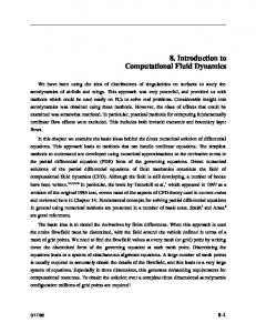


![[PDF] Download A Brief Introduction to Fluid Mechanics Full Edition](https://m.moam.info/img/260x300/pdf-download-a-brief-introduction-to-fluid-mechani_64789b69097c4786708d02d6.jpg)