Dec 15, 2018 - We start from the call-by-value version of the λµ Ëµ-calculus. ... inductive constructions for Coq [6], and Martin-Löf's type theory for Agda [24].
A Classical Sequent Calculus with Dependent Types Étienne Miquey
To cite this version: Étienne Miquey. A Classical Sequent Calculus with Dependent Types. ACM Transactions on Programming Languages and Systems (TOPLAS), ACM, In press.
HAL Id: hal-01519929 https://hal.inria.fr/hal-01519929v3 Submitted on 15 Dec 2018
HAL is a multi-disciplinary open access archive for the deposit and dissemination of scientific research documents, whether they are published or not. The documents may come from teaching and research institutions in France or abroad, or from public or private research centers.
L’archive ouverte pluridisciplinaire HAL, est destinée au dépôt et à la diffusion de documents scientifiques de niveau recherche, publiés ou non, émanant des établissements d’enseignement et de recherche français ou étrangers, des laboratoires publics ou privés.
A Classical Sequent Calculus with Dependent Types ÉTIENNE MIQUEY, INRIA, Équipe Gallinette Dependent types are a key feature of the proof assistants based on the Curry-Howard isomorphism. It is well-known that this correspondence can be extended to classical logic by enriching the language of proofs with control operators. However, they are known to misbehave in the presence of dependent types, unless dependencies are restricted to values. Moreover, while sequent calculi naturally support continuation-passing style interpretations, there is no such presentation of a language with dependent types. The main achievement of this paper is to give a sequent calculus presentation of a call-by-value language with a control operator and dependent types, and to justify its soundness through a continuation-passing style translation. ˜ We start from the call-by-value version of the λµ µ-calculus. We design a minimal language with a value restriction and a type system that includes a list of explicit dependencies to maintains type safety. We then show how to relax the value restriction and introduce delimited continuations to directly prove the consistency by means of a continuation-passing-style translation. Finally, we relate our calculus to a similar system by Lepigre, and present a methodology to transfer properties from this system to our own.
1 1.1
INTRODUCTION Control operators and dependent types
Originally created to deepen the connection between programming and logic, dependent types are now a key feature of numerous functional programming languages. From the point of view of programming, dependent types provide more precise types—and thus more precise specifications—to existing programs. From a logical perspective, they permit definitions of proof terms for statements like the full axiom of choice. Dependent types are provided by Coq or Agda, two of the most actively developed proof assistants. They both rely on constructive type theories: the calculus of inductive constructions for Coq [6], and Martin-Löf’s type theory for Agda [24]. Yet, both systems lack support for classical logic and more generally for side effects, which make them impractical as programming languages. In practice, effectful languages give the programmer a more explicit access to low-level control (that is: to the way the program is executed on the available hardware), and make some algorithms easier to implement. Common effects, such as the explicit manipulation of the memory, the generation of random numbers and input/output facilities are available in most practical programming languages (e.g., OCaml, C++, Python, Java). In 1990, Griffin discovered that the control operator call/cc (short for call with current continuation) could be typed by Peirce’s law ((A→ B) →A) →A) [15], thus extending the formulas-as-types interpretation. Indeed, Peirce’s law is known to imply, in an intuitionistic framework, all the other forms of classical reasoning (excluded middle, reductio ad absurdum, double negation elimination, etc.). This discovery opened the way for a direct computational interpretation of classical proofs, using control operators and their ability to backtrack. Several calculi were born from this idea, for example Parigot’s λµ-calculus [31], Barbanera and Berardi’s symmetric λ-calculus [3], Krivine’s ¯ µ-calculus ˜ λc -calculus [21], Curien and Herbelin’s λµ [7].
c b n a This work is licensed under a Creative Commons Attribution-ShareAlike 3.0 Unported License.
1:2
Étienne Miquey
Nevertheless, dependent types are known to misbehave in the presence of control operators, and lead to logical inconsistencies [17]. Since the same problem arises with a wider class of effects, it seems that we are facing the following dilemma: either we choose an effectful language (allowing us to write more programs) while accepting the lack of dependent types, or we choose a dependently typed language (allowing us to write finer specifications) and give up effects. Many works have tried to fill the gap between effectful programming languages and logic, by accommodating weaker forms of dependent types with computational effects (e.g., divergence, I/O, local references, exceptions). Amongst other works, we can cite the recent works by Ahman et al. [1], by Vákár [35, 36] or by Pédrot and Tabareau who proposed a systematical way to add effects to type theory [33]. Side effects—that are impure computations in functional programming—are often interpreted by means of monads. Interestingly, control operators can be interpreted similarly through the continuation monad, but the continuation monad generally lacks the properties necessary to fit these frameworks. Although dependent types and classical logic have been deeply studied separately, the problem of accommodating both features1 in one and the same system has not found a completely satisfying answer yet. Recent works from Herbelin [18] and Lepigre [22] proposed some restrictions on dependent types to make them compatible with a classical proof system, while Blot [5] designed a hybrid realizability model where dependent types are restricted to an intuitionistic fragment. 1.2
Call-by-value and value restriction
In languages enjoying the Church-Rosser property (like the λ-calculus or Coq), the order of evaluation is irrelevant, and any reduction path will ultimately lead to the same value. In particular, the call-by-name and call-by-value evaluation strategies will always give the same result. However, this is no longer the case in presence of side effects. Indeed, consider the simple case of a function applied to a term producing some side effects (for instance increasing a reference). In call-by-name, the computation of the argument is delayed to the time of its effective use, while in call-by-value the argument is reduced to a value before performing the application. If, for instance, the function never uses its argument, the call-by-name evaluation will not generate any side effect, and if it uses it twice, the side effect will occur twice (and the reference will have its value increased by two). On the contrary, in both cases the call-by-value evaluation generates the side effect exactly once (and the reference has its value increased by one). In this paper, we present a language following the call-by-value reduction strategy, which is as much a design choice as a goal in itself. Indeed, when considering a language with control operators (or other kinds of side effects), soundness often turns out to be subtle to preserve in call-by-value. The first issues in call-by-value in the presence of side effects were related to references [39] and polymorphism [16]. In both cases, a simple solution (but often unnecessarily restrictive in practice [14, 22]) to solve the inconsistencies consists in the introduction of a value restriction for the problematic cases, restoring then a sound type system. Recently, Lepigre presented a proof system providing dependent types and a control operator [22], whose consistency is preserved by means of a semantical value restriction defined for terms that behave as values up to observational equivalence. In the present work, we will rather use a syntactic restriction to a fragment of proofs 1 Aside
from strictly logical considerations as in [18], there are motivating examples of programs that could only be written and specified in such a setting. Consider for instance the infinite tape lemma that states that from any infinite sequence of natural numbers, one can extract either an infinite sequence of odd numbers, or an infinite sequence of even numbers. Its proof deeply relies on classical logic, and the corresponding program (which, given as input a stream of integers, returns a stream that consists either only of odd integers or only of even ones) can only be written in a classical setting and requires dependent types to be specified. See [23, Section 7.8] for more details.
A Classical Sequent Calculus with Dependent Types
1:3
that allows slightly more than values. As we will see, the restriction that arises naturally coincides with the negative-elimination-free fragment of Herbelin’s dPAω system [18]. 1.3
A sequent calculus presentation
The main achievement of this paper is to give a sequent calculus presentation2 of a call-by-value language with classical control and dependent types, and to justify its soundness through a ˜ continuation-passing style translation. Our calculus is an extension of the λµ µ-calculus [7] with dependent types. Amongst other motivations, such a calculus is close to an abstract machine, which makes it particularly suitable to define CPS translations or to be an intermediate language for compilation [8]. As a matter of fact, the original motivation for this work was the design of a program translation for Herbelin’s dPAω system (that already encompasses control operators and dependent types) to justify its soundness. However, this calculus was presented in a natural deduction style, making such a translation hard to obtain. We thus developed the framework presented in this paper to have an intermediate language more suitable for a continuation-passing style translation at our disposal. Additionally, while we consider in this paper the specific case of a calculus with classical logic, the sequent calculus presentation itself is responsible for another difficulty. As we will see, the usual ˜ call-by-value strategy of the λµ µ-calculus causes subject reduction to fail, which would already happen in an intuitionistic type theory. We claim that the solutions we give in this paper also works in the intuitionistic case. In particular, the system we develop might be a first step towards the adaption of the well-understood continuation-passing style translations for ML to design a (dependently) typed compilation of a system with dependent types such as Coq. 1.4
Delimited continuations and CPS translation
The main challenge in designing a sequent calculus with dependent types lies in the fact that the natural relation of reduction one would expect in such a framework is not safe with respect to types. As we will discuss in Section 2.6, the problem can be understood as a desynchronization of the type system with respect to the reduction. A simple solution, presented in Section 2, consists in the addition of an explicit list of dependencies in typing derivations. This has the advantage of leaving the computational part of the original calculus unchanged. However, it is not suitable for obtaining a continuation-passing style translation. We thus present a second way to solve this issue by introducing delimited continuations [2], which are used to force the purity needed for dependent types in an otherwise non purely functional language. It also justifies the relaxation of the value restriction and leads to the definition of the negative-elimination-free fragment (Section 3). In addition, it allows for the design, in Section 4, of a continuation-passing style translation that preserves dependent types and permits us to prove the soundness of our system. Finally, it also provides us with a way to embed our calculus into Lepigre’s calculus [22], as we shall see in Section 5. This embedding has in particular the benefit of furnishing us with a realizability interpretation for free. 1.5
Contributions of the paper
Our main contributions in this paper can be listed as follows: • We soundly combine dependent types and control operators by means of a syntactic restriction to the negative-elimination-free fragment; 2 In
˜ the sense of a formulas-as-types interpretation of a sequent calculus à la Hilbert (as Curien-Herbelin’s λµ µ-calculus [7] or Munch-Maccagnoni’s system L [29]), as opposed to traditional type systems given in a natural deduction style.
1:4
Étienne Miquey • We give a sequent calculus presentation and solve the type-soundness issues it raises in two different ways; • Our first solution simply relies on a list of dependencies that is added to the type system • Our second solution uses delimited continuations to ensure consistency with dependent types and provides us with a CPS translation (carrying dependent types) to a calculus without control operator; • We relate our system to Lepigre’s calculus, which gives us a realizability interpretation for free and offers an additional way of proving the consistency of our system.
This paper is an extended and revised version of the article presented at ESOP 2017 [26]. 2
A MINIMAL CLASSICAL LANGUAGE WITH DEPENDENT TYPES ˜ 2.1 A short primer to the λµ µ-calculus ˜ We recall here the spirit of the λµ µ-calculus, for further details and references please refer to the original article [7]. The syntax and reduction rules (parameterized over a subset of proofs V ˜ can be read as a context and a subset of evaluation contexts E) are given in Figure 1, where µa.c let a = [ ] in c. A command ⟨p||e⟩ can be understood as a state of an abstract machine, representing the evaluation of a proof p (the program) against a co-proof e (the stack) that we call context. The µ operator comes from Parigot’s λµ-calculus [31], µα binds a context to a context variable α in the ˜ binds a proof to some proof variable a. same way that µa ˜ The λµ µ-calculus can be seen as a proof-as-program correspondence between sequent calculus and abstract machines. Right introduction rules correspond to typing rules for proofs, while left introduction are seen as typing rules for evaluation contexts. In contrast with Gentzen’s original ˜ presentation of sequent calculus, the type system of the λµ µ-calculus explicitly identifies at any time which formula is being worked on. In a nutshell, this presentation distinguishes between three kinds of sequents: (1) sequents of the form Γ ⊢ p : A | ∆ for typing proofs, where the focus is put on the (right) formula A; (2) sequents of the form Γ | e : A ⊢ ∆ for typing contexts, where the focus is put on the (left) formula A; (3) sequents of the form c : (Γ ⊢ ∆) for typing commands, where no focus is set. In a right (resp. left) sequent Γ ⊢ p : A | ∆, the singled out formula3 A reads as the conclusion “where the proof shall continue” (resp. hypothesis “where it happened before”). For example, the left introduction rule of implication can be seen as a typing rule for pushing an element q on a stack e leading to the new stack q · e: Γ ⊢q :A | ∆ Γ |e :B ⊢∆ →l Γ | q ·e :A → B ⊢ ∆ As for the reduction rules, we can see that there is a critical pair if V and E are not restricted enough: ˜ .c ′] ←− ⟨µα .c || µx ˜ .c ′⟩ −→ c ′[x := µα .c]. c[α := µx The difference between call-by-name and call-by-value can be characterized by how this critical pair4 is solved, by defining V and E such that the two rules do not overlap. Defining the subcategories 3 This
formula is often referred to as the formula in the stoup, a terminology due to Girard. that this critical pair can be also interpreted in terms of non-determinism. Indeed, we can define a fork instruction ˜ by ⋔≜ λab .µα .⟨µ_⟨a ||α ⟩ || µ_.⟨b ||α ⟩⟩, which verifies indeed that ⟨⋔ ||p0 · p1 · e⟩ → ⟨p0 ||e⟩ and ⟨⋔ ||p0 · p1 · e⟩ → ⟨p1 ||e⟩.
4 Observe
A Classical Sequent Calculus with Dependent Types
Proofs Contexts Commands
::= a | λa.p | µα .c ˜ ::= α | p · e | µa.c ::= ⟨p||e⟩
p e c
1:5 ˜ ⟨p|| µa.c⟩ → c[a := p] ⟨µα .c ||e⟩ → c[α := e] ˜ ⟨λa.p||u · e⟩ → ⟨u || µa.⟨p||e⟩⟩
(a) Syntax
(b) Reduction rules
Γ ⊢ t :A | ∆ Γ |e :A⊢∆ ⟨t ||e⟩ : (Γ ⊢ ∆) (a : A) ∈ Γ Γ⊢a:A| ∆ (α : A) ∈ ∆ Γ |α :A⊢∆
(Axr )
(Axl )
p∈V e∈E
Γ,a : A ⊢ p : B | ∆ Γ ⊢ λa.p : A → B | ∆
(Cut)
c : (Γ ⊢ ∆,α : A) Γ ⊢ µα .c : A | ∆
(→r )
Γ ⊢p :A | ∆ Γ |e:B⊢∆ Γ | p ·e :A → B ⊢ ∆
(→l )
(µ )
c : (Γ,a : A ⊢ ∆) ˜ Γ | µa.c :A⊢∆
( µ˜ )
(c) Typing rules ˜ Fig. 1. The λµ µ-calculus
of values V ⊂ p and co-values E ⊂ e by: (Values)
V ::= a | λa.p
(Co-values)
E ::= α | q · e
the call-by-name evaluation strategy amounts to the case where V ≜ Proofs and E ≜ Co-values, while call-by-value corresponds to V ≜ Values and E ≜ Contexts. Both strategies can also be characterized through different CPS translations [7, Section 8]. ˜ Remark 2.1 (Application). The reader unfamiliar with the λµ µ-calculus might be puzzled by the absence of a syntactic construction for the application of proof terms. Intuitively, the usual application p q of the λ-calculus is replaced by the application of the proof p to a stack of the shape q · e as in an abstract machine5 . The usual application can thus be recovered through the following shorthand: p q ≜ µα .⟨p||q · α⟩ Finally, it is worth noting that the µ binder is a control operator, since it allows for catching evaluation contexts and backtracking further in the execution. This is the key ingredient that makes ˜ the λµ µ-calculus a proof system for classical logic. To illustrate this, let us draw the analogy with the call/cc operator of Krivine’s λc -calculus [21]. Let us define the following proof terms: call/cc ≜ λa.µα .⟨a||k α · α⟩
k e ≜ λa ′ .µβ .⟨a ′ ||e⟩
The proof k e can be understood as a proof term where the context e has been encapsulated. As expected, call/cc is a proof for Peirce’s law (see Figure 2), which is known to imply other forms of classical reasoning (e.g., the law of excluded middle, the double negation elimination). Let us observe the behavior of call/cc (in call-by-name evaluation strategy, as in Krivine λc -calculus): in front of a context of the shape q · e with e of type A, it will catch the context e thanks to the µα binder and reduce as follows: ⟨λa.µα .⟨a||k α · α⟩||q · e⟩ 5 To
˜ → ⟨q|| µa.⟨µα .⟨a||k α · α⟩||e⟩⟩ → ⟨µα .⟨q||k α · α⟩||e⟩ → ⟨q||k e · e⟩
pursue the analogy with the λ-calculus, the rest of the stack e can be viewed as a context C e [ ] surrounding the application p q, the command ⟨p ||q · e⟩ thus being identified with the term C e [p q]. Similarly, the whole stack can be seen as the context Cq·e [ ] = C e [[ ]q], whence the terminology.
1:6
Étienne Miquey (Axr )
(Axl )
•,a ′ : A ⊢ a ′ : A | • • | α : A ⊢ α : A, • (Cut) ⟨a ′ ||α⟩ : (•,a ′ : A ⊢ α : A, β : B) (µ ) •,a ′ : A ⊢ µβ .⟨a ′ ||α⟩ : B | α : A (→r ) (Axl ) • ⊢ λa ′ .µβ .⟨a ′ ||α⟩ : A → B | α : A |α :A⊢α :A (→l ) (Axr ) a : (A → B) → A ⊢ a : (A → B) → A | • • | λa ′ .µβ .⟨a ′ ||α⟩ · α : (A → B) → A ⊢ α : A (Cut) ⟨a||λa ′ .µβ .⟨a ′ ||α⟩ · α⟩ : (a : (A → B) → A ⊢ α : A) (µ ) a : (A → B) → A ⊢ µα .⟨a||λa ′ .µβ .⟨a ′ ||α⟩ · α⟩ : A | (→r ) ⊢ λa.µα .⟨a||λa ′ .µβ .⟨a ′ ||α⟩ · α⟩ : ((A → B) → A) → A | (where • is used to shorten useless parts of typing contexts.)
Fig. 2. Proof term for Peirce’s law
We notice that the proof term k e = λa ′ .µβ .⟨a ′ ||e⟩ on top of the stack (which, if e was of type A, is of type A → B, see Figure 2) contains a second binder µβ. In front of a stack q ′ · e ′, this binder will now catch the context e ′ and replace it by the former context e: ⟨λa ′ .µβ .⟨a ′ ||e⟩||q ′ · e ′⟩
→
˜ ′ .⟨µβ .⟨a ′ ||e⟩||e ′⟩⟩ ⟨q ′ || µa
⟨µβ .⟨q ′ ||e⟩||e ′⟩
→
→
⟨q ′ ||e⟩
This computational behavior corresponds exactly to the usual reduction rule for call/cc in the Krivine machine [21]: call/cc ⋆ t · π ≻ t ⋆ k π · π kπ ⋆ t · π ′ ≻ t ⋆ π 2.2
Inconsistency of classical logic with dependent types
The simultaneous presence of classical logic (i.e. of a control operator) and dependent types is known to cause a degeneracy of the domain of discourse. Let us shortly recap the argument of Herbelin highlighting this phenomenon [17]. Let us adopt here a stratified presentation of dependent types, by syntactically distinguishing terms—that represent mathematical objects—from proof terms—that represent mathematical proofs. In other words, we syntactically separate the categories corresponding to witnesses and proofs in dependent sum types. Consider a minimal logic of strong existentials and equality, whose formulas, terms (only representing natural number) and proofs are defined as follows: Formulas Terms Proofs
A,B t,u p,q
::= t = u | ∃x N .A ::= n | wit p | x ::= refl | subst p q | (t,p) | prf p
(n ∈ N)
Let us explain the different proof terms by presenting their typing rules. First of all, the pair (t,p) is a proof for an existential formula ∃x N .A where t is a witness for x and p is a certificate for A[t/x]. This implies that both formulas and proofs are dependent on terms, which is usual in mathematics. What is less usual in mathematics is that, as in Martin-Löf’s type theory, dependent types also allow for terms (and thus for formulas) to be dependent on proofs, by means of the constructors wit p and prf p. Typing rules are given with separate typing judgments for terms, which can only be of type N: Γ ⊢ p : A(t ) Γ ⊢ (t,p) :
Γ ⊢t :N ∃x N.A
(∃I )
Γ ⊢ (t,p) : ∃x N.A Γ ⊢ prf p : A[wit p/x]
(prf )
Γ ⊢ t : ∃x N.A Γ ⊢ wit t : N
(wit)
n∈N Γ ⊢n:N
A Classical Sequent Calculus with Dependent Types
1:7
Then, refl is a proof term for equality, and subst p q allows us to use a proof of an equality t = u to convert a formula A(t ) into A(u): t →u Γ ⊢ refl : t = u
Γ ⊢ p : t = u Γ ⊢ q : B[t] Γ ⊢ subst p q : B[u]
(refl)
(subst)
The reduction rules for this language, which are safe with respect to typing, are then: wit (t,p) → t
prf (t,p) → p
subst refl p → p
Starting from this (sound) minimal language, Herbelin showed that its classical extension with the control operators call/cck and throw k (that are similar to those presented in the previous section) permits to derive a proof of 0 = 1 [17]. The call/cck operator, which is a binder for the variable k, is intended to catch its surrounding evaluation context. On the contrary, throw k discards the current context and restores the context captured by call/cck . The addition to the type system of the typing rules for these operators: Γ,k : ¬A ⊢ p : A Γ ⊢ call/cck p : A
Γ,k : ¬A ⊢ p : A Γ,k : ¬A ⊢ throw k p : B
allows the definition of the following proof: p0 ≜ call/cck (0, throw k (1, refl)) : ∃x N.x = 1 Intuitively such a proof catches the context, gives 0 as witness (which is incorrect), and a certificate that will backtrack and give 1 as witness (which is correct) with a proof of the equality. If, besides, the following reduction rules6 are added: wit (call/cck p) call/cck t
→ call/cck (wit (p[k (wit { })/k])) → t
(k < FV (t ))
then we can formally derive a proof of 1 = 0. Indeed, the term wit p0 will reduce to call/cck 0, which itself reduces to 0. The proof term refl is thus a proof of wit p0 = 0, and we obtain the following proof of 1 = 0: ⊢ p0 : ∃x N .x = 1 wit p0 → 0 (prf ) ⊢ prf p0 : wit p0 = 1 ⊢ refl : wit p0 = 0 ⊢ subst (prf p0 ) refl : 1 = 0
(refl) (subst)
The bottom line of this example is that the same proof p0 is behaving differently in different contexts thanks to control operators, causing inconsistencies between the witness and its certificate. The easiest and usual approach (in natural deduction) to prevent this is to impose a restriction to values (which are already reduced) for proofs appearing inside dependent types and within the operators wit and prf , together with a call-by-value discipline. In the present example, this would prevent us from writing wit p0 and prf p0 . 6 Technically this requires to extend the language to authorize the construction of terms call/cc t and of proofs throw t . k The first rule expresses that call/cck captures the context wit { } and replaces every occurrence of throw k t with throw k (wit t ). The second one just expresses the fact that call/cck can be dropped when applied to a term t which does not contain the variable k .
1:8 2.3
Étienne Miquey A minimal language with value restriction
In this section, we will focus on value restriction in a similar framework, and show that the obtained proof system is coherent. We will then see, in Section 3, how to relax this constraint. We follow here the stratified presentation7 from the previous section. We place ourselves in the framework of ˜ the λµ µ-calculus to which we add: • a language of terms which contain an encoding8 of the natural numbers, • proof terms (t,p) to inhabit the strong existential ∃x N.A together with the first and second projections, called respectively wit (for terms) and prf (for proofs), • a proof term refl for the equality of terms and a proof term subst for the convertibility of types over equal terms. For simplicity reasons, we will only consider terms of type N throughout this paper. We address the question of extending the domain of terms in Section 6.2. The syntax of the corresponding system, that we call dL, is given by: Terms Proof terms Proof values Contexts Commands
t p V e c
::= ::= ::= ::= ::=
x | n | wit V V | µα .c | (t,p) | prf V | subst p q a | λa.p | λx .p | (t,V ) | refl ˜ α | p · e | t · e | µa.c ⟨p||e⟩
(n ∈ N)
The formulas are defined by: Formulas
A,B
::=
⊤ | ⊥ | t = u | ∀x N .A | ∃x N .A | Πa:A B.
Note that we included a dependent product Πa:A B at the level of proof terms, but that in the case where a < FV (B) this amounts to the usual implication A → B. 2.4
Reduction rules
As explained in Section 2.2, a backtracking proof might give place to different witnesses and proofs according to the context of reduction, leading to inconsistencies [17]. The substitution at different places of a proof which can backtrack, as the call-by-name evaluation strategy does, is thus an unsafe operation. On the contrary, the call-by-value evaluation strategy forces a proof to reduce first to a value (thus furnishing a witness) and to share this value amongst all the commands. In particular, this maintains the value restriction along reduction, since only values are substituted. The reduction rules, defined in Figure 3 (where t → t ′ denotes the reduction of terms and c ⇝ c ′ the reduction of commands), follow the call-by-value evaluation principle. In particular one can see that whenever a command is of the shape ⟨C[p]||e⟩ where C[p] is a proof built on top of p which is ˜ not a value, it reduces to ⟨p|| µa.⟨C[a]||e⟩⟩, opening the construction to evaluate p 9 . Additionally, we denote by A ≡ B the transitive-symmetric closure of the relation A ▷ B, defined as a congruence over term reduction (i.e. if t → t ′ then A[t] ▷ A[t ′]) and by the rules: 0=0▷⊤ S (t ) = 0 ▷ ⊥ 7 This
0 = S (u) ▷ ⊥ S (t ) = S (u) ▷ t = u
design choice is usually a matter of taste and might seem unusual for some readers. However, it has the advantage of exhibiting the different treatments for terms and proofs through the CPS in the next sections. 8 The nature of the representation is irrelevant here as we will not compute over it. We can for instance add one constant for each natural number. 9 The reader might recognize the rule (ς ) of Wadler’s sequent calculus [38].
A Classical Sequent Calculus with Dependent Types ⟨µα .c ||e⟩ ˜ ⟨V || µa.c⟩ ⟨λa.p||q · e⟩ ⟨λx .p||t · e⟩
⇝ ⇝ ⇝ ⇝
c[e/α] c[V /a] ˜ ⟨q|| µa.⟨p||e⟩⟩ ⟨p[t/x]||e⟩
wit (t,V ) → t
⟨(t,p)||e⟩ ⟨prf (t,V )||e⟩ ⟨subst p q||e⟩ ⟨subst refl q||e⟩
1:9 ⇝ ⇝ ⇝ ⇝
˜ ⟨p|| µa.⟨(t,a)||e⟩⟩ ⟨V ||e⟩ ˜ ⟨p|| µa.⟨subst a q||e⟩⟩ ⟨q||e⟩
(p < Values) (p < Values)
t → t ′ ⇒ c[t] ⇝ c[t ′] Fig. 3. Reduction rules of dL
2.5
Typing rules
As we explained before, in this section we limit ourselves to the simple case where dependent types are restricted to values, to make them compatible with classical logic. But even with this restriction, defining the type system in the most naive way leads to a system in which subject reduction will fail. Having a look at the β-reduction rule gives us an insight of what happens. Let us imagine ˜ that the type system of the λµ µ-calculus has been extended to allow dependent products instead of implications. and consider a proof λa.p : Πa:A B in front of a context q · e : Πa:A B. A typing derivation of the corresponding command would be of the form: Πp Πq Πe Γ,a : A ⊢ p : B | ∆ Γ ⊢ q : A | ∆ Γ | e : B[q/a] ⊢ ∆ (→r ) Γ ⊢ λa.p : Πa:A B | ∆ Γ | q · e : Πa:A B ⊢ ∆ (Cut) ⟨λa.p||q · e⟩ : Γ ⊢ ∆
(→l )
while this command would reduce as follows: ˜ ⟨λa.p||q · e⟩ ⇝ ⟨q|| µa.⟨p||e⟩⟩. On the right-hand side, we see that p, whose type is B[a], is now cut with e whose type is B[q]. Consequently, we are not able to derive a typing judgment10 for this command anymore: � | ∆ Γ,a : A | e : B[q] B[a] Γ,a : A ⊢ p : � �� ⊢ ∆ Mismatch Πq ⟨p||e⟩ : Γ,a : A ⊢ ∆ ( µ˜ ) ˜ Γ ⊢q :A | ∆ Γ | µa.⟨p||e⟩ :A⊢∆ (Cut) ˜ ⟨q|| µa.⟨p||e⟩⟩ :Γ⊢∆ The intuition is that in the full command, a has been linked to q at a previous level of the typing judgment. However, the command is still safe, since the head-reduction imposes that the command ⟨p||e⟩ will not be executed before the substitution of a by q 11 is performed, and by then the problem would be solved. This phenomenon can be seen as a desynchronization of the typing process with respect to computation. The synchronization can be re-established by making explicit a list of dependencies σ in the typing rules, which links µ˜ variables (here a) to the associated proof term on 10 Observe
that the problem here arises independently of the value restriction (that is whether we consider that q is a value or not), and is peculiar to the sequent calculus presentation. 11 Note that even if we were not restricting ourselves to values, this would still hold: if at some point the command ⟨p ||e⟩ is executed, it is necessarily the case that q has produced a value to substitute for a.
1:10
Étienne Miquey Γ ⊢ p : A | ∆; σ (a : A) ∈ Γ Γ ⊢ a : A | ∆; σ
Γ | e : B ⊢ ∆; σ {·|p} ⟨p||e⟩ : Γ ⊢ ∆; σ
(α : A) ∈ ∆ Γ | α : A ⊢ ∆; σ {·|p}
(Axr )
c : (Γ,a : A ⊢ ∆; σ {a|p}) ˜ Γ | µa.c : A ⊢ ∆; σ {·|p} Γ ⊢ q : A | ∆; σ Γ,x : N ⊢ p : A | ∆; σ Γ ⊢ λx .p : ∀x N.A | ∆; σ Γ ⊢ t : N | ∆; σ
c : (Γ ⊢ ∆,α : A; σ ) Γ ⊢ µα .c : A | ∆; σ
Γ,a : A ⊢ p : B | ∆; σ Γ ⊢ λa.p : Πa:A B | ∆; σ
( µ˜ )
(µ )
(→r )
(→l )
Γ ⊢ t : N ⊢ ∆; σ Γ | e : A[t/x] ⊢ ∆; σ {·|†} Γ | t · e : ∀x N.A ⊢ ∆; σ {·|p}
(∀r )
Γ ⊢ p : A(t ) | ∆; σ
Γ ⊢ p : A | ∆; σ A ≡ B Γ ⊢ p : B | ∆; σ
(≡r )
n∈N Γ ⊢ n : N | ∆; σ
(∀l )
Γ ⊢ p : ∃x N.A(x ) | ∆; σ p ∈ D prf Γ ⊢ prf p : A(wit p) | ∆; σ
(∃r )
Γ ⊢ p : t = u | ∆; σ Γ ⊢ q : B[t/x] | ∆; σ Γ ⊢ subst p q : B[u/x] | ∆; σ (Axt )
(Axl )
(Cut)
Γ | e : B[q/a] ⊢ ∆; σ {·|†} q < D → a < FV (B) Γ | q · e : Πa:A B ⊢ ∆; σ {·|p}
Γ ⊢ (t,p) : ∃x N.A(x ) | ∆; σ
Γ,x : N ⊢ x : N | ∆; σ
B ∈ Aσ
Γ | e : A ⊢ ∆; σ A ≡ B Γ | e : B ⊢ ∆; σ (subst)
(Axn )
(≡l )
Γ ⊢ t : N | ∆; σ Γ ⊢ refl : t = t | ∆; σ
(refl)
Γ ⊢ p : ∃x .A(x ) | ∆; σ p ∈ D Γ ⊢ wit p : N | ∆; σ
(wit)
Fig. 4. Typing rules of dL
the left-hand side of the command (here q). We can now obtain the following typing derivation: Πp Πe Γ,a : A ⊢ p : B[a] | ∆ Γ,a : A | e : B[q] ⊢ ∆; σ {a|q}{·|p} Πq ⟨p||e⟩ : Γ,a : A ⊢ ∆; σ {a|q} ( µ˜ ) ˜ Γ ⊢q :A | ∆ Γ | µa.⟨p||e⟩ : A ⊢ ∆; σ {.|q} (Cut) ˜ ⟨q|| µa.⟨p||e⟩⟩ : Γ ⊢ ∆; σ
(Cut)
Formally, we denote by D the set of proofs we authorize in dependent types, and define it for the moment as the set of values: D ≜ V. We define a list of dependencies σ as a list binding pairs of proof terms12 : σ ::= ε | σ {p|q}, 12 In
practice we will only bind a variable with a proof term, but it is convenient for proofs to consider this slightly more general definition.
A Classical Sequent Calculus with Dependent Types
1:11
and we define Aσ as the set of types that can be obtained from A by replacing all (or none) occurrences of p by q for each binding {p|q} in σ such that q ∈ D: Aσ ∪ (A[q/p])σ if q ∈ D Aσ {p |q } ≜ A σ otherwise. The list of dependencies is filled while going up in the typing tree, and it can be used when typing a command ⟨p||e⟩ to resolve a potential inconsistency between their types: Aε ≜ {A}
Γ ⊢ p : A | ∆; σ
Γ | e : B ⊢ ∆; σ {·|p} ⟨p||e⟩ : Γ ⊢ ∆; σ
B ∈ Aσ
(Cut)
Remark 2.2. The reader familiar with explicit substitutions [11] can think of the list of dependencies as a fragment of the substitution that is available when a command c is reduced. Another remark is that the design choice for the (Cut) rule is arbitrary, in the sense that we chose to check whether B is in Aσ . We could equivalently have checked whether the condition σ (A) = σ (B) holds, where σ (A) refers to the type A where for each binding {p|q} ∈ σ with q ∈ D, all the occurrences of p have been replaced by q. Furthermore, when typing a stack with the (→l ) and (∀l ) rules, we need to drop the open binding in the list of dependencies13 . We introduce the notation Γ | e : A ⊢ ∆; σ {·|†} to denote that the dependency to be produced is irrelevant and can be dropped. This trick spares us from defining a second type of sequents Γ | e : A ⊢ ∆; σ to type contexts when dropping the (open) binding {·|p}. Alternatively, one can think of † as any proof term not in D, which is the same with respect to the list of dependencies. The resulting set of typing rules is given in Figure 4, where we assume that every variable bound in the typing context is bound only once (proofs and contexts are considered up to α-conversion). Note that we work with two-sided sequents here to stay as close as possible to the original ˜ presentation of the λµ µ-calculus [7]. In particular this means that a type in ∆ might depend on a variable previously introduced in Γ and vice versa, so that the split into two contexts makes us lose track of the order of introduction of the hypotheses. In the sequel, to be able to properly define a typed CPS translation, we consider that we can unify both contexts into a single one that is coherent with respect to the order in which the hypotheses have been introduced. Example 2.3. The proof p1 ≜ subst (prf p0 ) refl which was of type 1 = 0 in Section 2.2 is now incorrect since the backtracking proof p0 , defined by µα .(0, µ_.⟨(1, refl)||α⟩) in our framework, is ˜ not a value in D. The proof p1 should rather be defined by14 µα .⟨p0 || µa.⟨subst (prf a) refl||α⟩⟩ which can only be given the type 1 = 1. 2.6
Subject reduction
We start by giving a few technical lemmas that will be used for proving subject reduction. First, we will show that typing derivations allow weakening on the lists of dependencies. For this purpose, we introduce the notation σ ⇛ σ ′ to denote that whenever a judgment is derivable with σ as list of dependencies, then it is derivable using σ ′: σ ⇛ σ ′ ≜ ∀c ∀Γ ∀∆.(c : (Γ ⊢ ∆; σ ) ⇒ c : (Γ ⊢ ∆; σ ′ )). 13 It
˜ .c⟩ with {· |p }, the “correct” dependency within c is easy to convince ourselves that when typing a command ⟨p ||q · µa should be {a |µα ⟨p ||q · α ⟩}, where the right proof is not a value. Furthermore, this dependency is irrelevant since there is no way to produce such a command where a type adjustment with respect to a needs to be made in c. 14 That is to say let a = p in subst (prf a) refl in natural deduction. 0
1:12
Étienne Miquey
This clearly implies that the same property holds when typing evaluation contexts, i.e. if σ ⇛ σ ′ then σ can be replaced by σ ′ in any typing derivation for any context e. Lemma 2.4 (Dependencies weakening). For any list of dependencies σ we have: 1. ∀V .(σ {V |V } ⇛ σ )
2. ∀σ ′ .(σ ⇛ σσ ′ )
Proof. The first statement is obvious. The proof of the second one is straightforward from the fact that for any p and q, by definition Aσ ⊂ Aσ {p |q } . □ As a corollary, we get that † can indeed be replaced by any proof term when typing a context. Corollary 2.5. If σ ⇛ σ ′, then for any p,e, Γ, ∆: Γ | e : A ⊢ ∆; σ {·|†} ⇒ Γ | e : A ⊢ ∆; σ ′ {·|p}. ˜ (other cases are trivial), then we have c : Γ ⊢ ∆; σ {a|†}. Proof. Assume that e is of the form µa.c By definition of † and from the hypothesis, we get that σ {a|†} ⇛ σ ′, i.e. that c : Γ ⊢ ∆; σ ′ is derivable. By applying the previous Lemma, we get that c : Γ ⊢ ∆; σ ′ {a|p} is derivable for any proof p, whence the result. □ We first state the usual lemmas that guarantee the safety of terms (resp. values, contexts) substitution. Lemma 2.6 (Safe term substitution). If Γ ⊢ t : N | ∆; ε then: (1) c : (Γ,x : N, Γ ′ ⊢ ∆; σ ) ⇒ c[t/x] : (Γ, Γ ′[t/x] ⊢ ∆[t/x]; σ [t/x]), (2) Γ,x : N, Γ ′ ⊢ q : B | ∆; σ ⇒ Γ, Γ ′[t/x] ⊢ q[t/x] : B[t/x] | ∆[t/x]; σ [t/x], (3) Γ,x : N, Γ ′ | e : B ⊢ ∆; σ ⇒ Γ, Γ ′[t/x] | e[t/x] : B[t/x] ⊢ ∆[t/x]; σ [t/x], (4) Γ,x : N, Γ ′ ⊢ u : N | ∆; σ ⇒ Γ, Γ ′[t/x] ⊢ u[t/x] : N | ∆[t/x]; σ [t/x]. Lemma 2.7 (Safe value substitution). If Γ ⊢ V : A | ∆; ε then: (1) c : (Γ,a : A, Γ ′ ⊢ ∆; σ ) ⇒ c[V /a] : (Γ, Γ ′[V /a] ⊢ ∆[V /a]; σ [V /a]), (2) Γ,a : A, Γ ′ ⊢ q : B | ∆; σ ⇒ Γ, Γ ′[V /a] ⊢ q[V /a] : B[V /a] | ∆[V /a]; σ [t/x], (3) Γ,a : A, Γ ′ | e : B ⊢ ∆; σ ⇒ Γ, Γ ′[V /a] | e[V /a] : B[V /a] ⊢ ∆[V /a]; σ [V /a], (4) Γ,a : A, Γ ′ ⊢ u : N | ∆; σ ⇒ Γ, Γ ′[V /a] ⊢ u[V /a] : N | ∆[V /a]; σ [V /a]. Lemma 2.8 (Safe context substitution). If Γ | e : A ⊢ ∆; ε then: (1) c : (Γ ⊢ ∆,α : A, ∆ ′; σ ) ⇒ c[e/α] : (Γ ⊢ ∆, ∆ ′; σ ), (2) Γ ⊢ q : B | ∆,α : A, ∆ ′; σ ⇒ Γ ⊢ q[e/α] : B | ∆, ∆ ′; σ , (3) Γ | e : B ⊢ ∆,α : A, ∆ ′; σ ⇒ Γ | e[e/α] : B ⊢ ∆, ∆ ′; σ , (4) Γ ⊢ u : N | ∆,α : A, ∆ ′; σ ⇒ Γ ⊢ u : N | ∆, ∆ ′; σ ]. Proof. The proofs are done by induction on typing derivations.
□
We can now prove the preservation of typing through reduction, using the previous lemmas for rules which perform a substitution, and the list of dependencies to resolve local desynchronizations for dependent types. Theorem 2.9 (Subject reduction). If c,c ′ are two commands of dL such that c : (Γ ⊢ ∆; ε ) and c ⇝ c ′, then c ′ : (Γ ⊢ ∆; ε ). Proof. The proof is done by induction on the typing derivation of c : (Γ ⊢ ∆; ε), assuming that for each typing proof, the conversion rules are always pushed down and right as much as possible.
A Classical Sequent Calculus with Dependent Types
1:13
To save some space, we sometimes omit the list of dependencies when empty, writing c : Γ ⊢ ∆ instead of c : Γ ⊢ ∆; ε, and we denote the composition of consecutive rules (≡l ) as: Γ | e : B ⊢ ∆; σ Γ | e : A ⊢ ∆; σ
(≡l )
where the hypothesis A ≡ B is implicit. • Case ⟨λx .p||t · e⟩ ⇝ ⟨p[t/x]||e⟩. A typing proof for the command on the left-hand side is of the form: Πp Γ,x : N ⊢ p : A | ∆ Γ ⊢ λx .p : ∀x N.A | ∆
(∀r )
Πe Πt Γ ⊢ t : N | ∆ Γ | e : B[t/x] ⊢ ∆; {·|†} Γ | t · e : ∀x N.B ⊢ ∆; {·|λx .p}
Γ | t · e : ∀x N.A ⊢ ∆; {·|λx .p} ⟨λx .p||t · e⟩ : Γ ⊢ ∆
(∀l )
(≡l )
(Cut)
We first deduce A[t/x] ≡ B[t/x] from the hypothesis ∀x N.A ≡ ∀x N.B. Then, using the fact that Γ,x : N ⊢ p : A | ∆ and Γ ⊢ t : N | ∆, by Lemma 2.6 and the fact that ∆[t/x] = ∆, we get a proof Πp′ of Γ ⊢ p[t/x] : A[t/x] | ∆. We can thus build the following derivation: Πe Γ | e : B[t/x] ⊢ ∆; {·|p[t/x]} Γ ⊢ p[t/x] : A[t/x] | ∆ Γ | e : A[t/x] ⊢ ∆; {·|p[t/x]} ⟨p[t/x]||e⟩ : Γ ⊢ ∆ Πp′
(≡l ) (Cut)
using Corollary 2.5 to weaken the binding to p[t/x] in Πe . ˜ • Case ⟨λa.p||q · e⟩ ⇝ ⟨q|| µa.⟨p||e⟩⟩. A typing proof for the command on the left-hand side is of the form: Πp Γ,a : A ⊢ p : B | ∆ Γ ⊢ λa.p : Πa:A B | ∆
Πq Πe ′ Γ ⊢ q : A | ∆ Γ | e : B ′[q/a] ⊢ ∆; {·|†} Γ | q · e : Πa:A′ B ′ ⊢ ∆; {·|λa.p} (→r ) (≡l ) Γ | q · e : Πa:A B ⊢ ∆; {·|λa.p} (Cut) ⟨λa.p||q · e⟩ : Γ ⊢ ∆
If q < D, we define Bq′ ≜ B ′ which is the only type in B ′{a |q } . Otherwise, we define Bq′ ≜ B ′[q/a] which is a type in B ′{a |q } . In both cases, we can build the following derivation:
Πq Γ ⊢ q : A′ | ∆ Γ ⊢q :A | ∆
Πp Γ,a : A ⊢ p : B | ∆ Γ,a : A ⊢ p : B ′ | ∆ (≡l )
(≡r )
Πe Γ,a : A | e : Bq′ ⊢ ∆; {a|q}{·|p}
⟨p||e⟩ : Γ,a : A ⊢ ∆; {a|q} ˜ Γ | µa.⟨p||e⟩ : A ⊢ ∆; {.|q} ˜ ⟨q|| µa.⟨p||e⟩⟩ :Γ⊢∆
using Corollary 2.5 to weaken the dependencies in Πe .
( µ˜ ) (Cut)
Bq′ ∈ B ′{a |q }
(Cut)
1:14
Étienne Miquey
• Case ⟨µα .c ||e⟩ ⇝ c[e/α]. A typing proof for the command on the left-hand side is of the form: Πc Πe c : Γ ⊢ ∆,α : A (µ ) Γ ⊢ µα .c : A | ∆ Γ | e : A ⊢ ∆; {·|µα .c} ⟨µα .c ||e⟩ : Γ ⊢ ∆
(Cut)
We get a proof that c[e/α] : Γ ⊢ ∆ is valid by Lemma 2.8. ˜ • Case ⟨V || µa.c⟩ ⇝ c[V /a]. A typing proof for the command on the left-hand side is of the form: Πc c : Γ,a : A′ ⊢ ∆; {a|V } ˜ Γ | µa.c : A′ ⊢ ∆; {·|V } ΠV ˜ Γ ⊢V :A | ∆ Γ | µa.c : A ⊢ ∆; {·|V } ˜ ⟨V || µa.c⟩ :Γ⊢∆
( µ˜ ) (≡l ) (Cut)
We first observe that we can derive the following proof: ΠV Γ ⊢V :A | ∆ Γ ⊢ V : A′ | ∆
(≡l )
and we get a proof for c[V /a] : Γ ⊢ ∆; {V |V } by Lemma 2.7. We finally get a proof for c[V /a] : Γ ⊢ ∆ by Lemma 2.4. ˜ • Case ⟨(t,p)||e⟩ ⇝ ⟨p|| µa.⟨(t,a)||e⟩⟩, with p < V . A proof of the command on the left-hand side is of the form: Πt Γ ⊢t :N | ∆
Πp Γ ⊢ p : A[t/x] | ∆
Γ ⊢ (t,p) : ∃x N.A | ∆
Πe Γ | e : ∃x N.A ⊢ ∆; {·|(t,p)} ⟨(t,p)||e⟩ : Γ ⊢ ∆ (∃r )
(Cut)
We can build the following derivation: Π (t,a) ∃x N.A
Πp Γ ⊢ p : A[t/x] | ∆
(∃I )
∃x N.A
|∆ Γ,a : A[t/x] ⊢ (t,a) : Γ|e: ⟨(t,a)||e⟩ : Γ,a : A[t/x] ⊢ ∆; {a|p} ˜ Γ | µa.⟨(t,a)||e⟩ : A[t/x] ⊢ ∆; {·|p} ˜ ⟨p|| µa.⟨(t,a)||e⟩⟩ :Γ⊢∆
Πe ⊢ ∆; {a|p}{·|(t,a)}
(Cut)
( µ˜ ) (Cut)
where Π (t,a) is as expected, observing that since p < D, the binding {·|(t,p)} is the same as {·|†}, and we can apply Corollary 2.5 to weaken dependencies in Πe .
A Classical Sequent Calculus with Dependent Types
1:15
• Case ⟨prf (t,V )||e⟩ ⇝ ⟨V ||e⟩. This case is easy, observing that a derivation of the command on the left-hand side is of the form: ΠV Πt Γ ⊢ V : A(t ) | ∆ (∃r ) Γ ⊢ (t,V ) : ∃x N.A(x ) | ∆ Πe (prf ) Γ ⊢ prf (t,V ) : A(wit (t,V )) | ∆ Γ | e : A(wit (t,V )) ⊢ ∆; {·|†} ⟨prf (t,V )||e⟩ : Γ ⊢ ∆
(Cut)
Since by definition we have A(wit (t,V )) ≡ A(t ), we can derive: Πe Γ | e : A(wit (t,V )) ⊢ ∆; {·|V } ΠV (≡l ) Γ ⊢ V : A(t ) | ∆ Γ | e : A(t ) ⊢ ∆; {·|V } (Cut) ⟨prf (t,V )||e⟩ : Γ ⊢ ∆
• Case ⟨subst refl q||e⟩ ⇝ ⟨q||e⟩. This case is straightforward, observing that for any terms t,u, if we have refl : t = u, then A[t] ≡ A[u] for any A. ˜ • Case ⟨subst p q||e⟩ ⇝ ⟨p|| µa.⟨subst a q||e⟩⟩. This case is similar to the case ⟨(t,p)||e⟩. • Case c[t] ⇝ c[t ′] with t → t ′. Immediate by observing that by definition of the relation ≡, we have A[t] ≡ A[t ′] for any A. □ 2.7
Soundness
We here give a proof of the soundness of dL with a value restriction. The proof is based on an ˜ embedding into the λµ µ-calculus extended with pairs, whose syntax and rules are given in Figure 5. A more interesting proof through a continuation-passing translation is presented in Section 4. ˜ We first show that typed commands of dL normalize by translation to the simply-typed λµ µcalculus with pairs (i.e. extended with proofs of the form (p1 ,p2 ) and contexts of the form µ˜ (a 1 ,a 2 ).c). We do not consider here a particular reduction strategy, and take ↣ to be the contextual closure of the rules given in Figure 5. The translation essentially consists in erasing the dependencies in types15 , turning the dependent products into arrows and the dependent sum into a pair. The erasure procedure is defined by: (∀x N.A) ∗ ≜ N → A∗ (∃x N.A) ∗ ≜ N ∧ A∗ (Πa:A B) ∗ ≜ A∗ → B ∗
⊤∗ ≜ N → N ⊥∗ ≜ N → N (t = u) ∗ ≜ N → N
and the corresponding translation for terms, proofs, contexts and commands is given by: 15 The
use of erasure functions is a very standard technique in the systems of the λ-cube, see for instance [32] or [37].
1:16
Étienne Miquey
Proofs Values Contexts Commands
p V e c
::= V | µα .c | (p1 ,p2 ) ::= a | λa.p | (V1 ,V2 ) ˜ ::= α | p · e | µa.c | µ˜ (a 1 ,a 2 ).c ::= ⟨p||e⟩
Γ ⊢ p 1 : A1 | ∆ Γ ⊢ p 2 : A2 | ∆ Γ ⊢ (p1 ,p2 ) : A1 ∧ A2 | ∆ c : Γ,a 1 : A1 ,a 2 : A2 ⊢ ∆ Γ | µ˜ (a 1 ,a 2 ).c : A1 ∧ A2 ⊢ ∆
(a) Syntax
(∧r )
(∧l )
(b) Typing rules ⟨(p1 ,p2 )|| µ˜ (a 1 ,a 2 ).c⟩ ↣ c[p1 /a 1 ][p2 /a 2 ] µα .⟨p||α⟩ ↣ p ˜ µa.⟨a||e⟩ ↣ e
⟨µα .c ||e⟩ ↣ c[e/α] ˜ ⟨λa.p||q · e⟩ ↣ ⟨q|| µa.⟨p||e⟩⟩ ˜ ⟨p|| µa.c⟩ ↣ c[p/a]
(c) Reduction rules ˜ Fig. 5. λµ µ-calculus with pairs
⟨p||e⟩∗ ≜ ⟨p ∗ ||e ∗ ⟩ α∗ (t · e) ∗ (q · e) ∗ ∗ ˜ ( µa.c)
≜α ≜ t ∗ · e∗ ≜ q∗ · e ∗ ˜ ∗ ≜ µa.c
x∗ n¯∗ (wit p) ∗ a∗ refl∗
≜x ≜ n¯ ≜ π1 (p ∗ ) ≜a ≜ λx .x
(λa.p) ∗ (λx .p) ∗ (µα .c) ∗ (prf p) ∗ (t,p) ∗
≜ λa.p ∗ ≜ λx .p ∗ ≜ µα .c ∗ ≜ π2 (p ∗ ) ∗ ,a)||α⟩⟩ ˜ ≜ µα .⟨p ∗ || µa.⟨(t
(subst V q) ∗ ≜ µα .⟨q ∗ ||α⟩ ˜ .⟨µα .⟨q ∗ ||α⟩||α⟩⟩ (subst p q) ∗ ≜ µα .⟨p ∗ || µ_ (p < V ) where πi (p) ≜ µα .⟨p|| µ˜ (a 1 ,a 2 ).⟨a 1 ||α⟩⟩. The term n¯ is defined as any encoding of the natural number n with its type N∗ , the encoding being irrelevant here as long as n¯ ∈ V . Note that we translate differently subst V q and subst p q to simplify the proof of Proposition 2.12. We first show that the erasure procedure is adequate with respect to the previous translation. Lemma 2.10. The following holds for any types A and B: (1) For any terms t and u, (A[t/u]) ∗ = A∗ . (2) For any proofs p and q, (A[p/q]) ∗ = A∗ . (3) If A ≡ B then A∗ = B ∗ . (4) For any list of dependencies σ , if A ∈ B σ , then A∗ = B ∗ . Proof. Straightforward: (1) and (2) are direct consequences of the erasure of terms (and thus proofs) from types. (3) follows from (1),(2) and the fact that (t = u) ∗ = ⊤∗ = ⊥∗ . (4) follows from (2). □ We can extend the erasure procedure to typing contexts, and show that it is adequate with respect to the translation of proofs. Proposition 2.11. The following holds for any contexts Γ, ∆ and any type A: (1) For any command c, if c : Γ ⊢ ∆; σ , then c ∗ : Γ ∗ ⊢ ∆∗ . (2) For any proof p, if Γ ⊢ p : A | ∆; σ , then Γ ∗ ⊢ p ∗ : A∗ | ∆∗ . (3) For any context e, if Γ | e : A ⊢ ∆; σ , then Γ ∗ | e ∗ : A∗ ⊢ ∆∗ . Proof. By induction on typing derivations. The fourth item of the previous lemma shows that the list of dependencies becomes useless: since A ∈ B σ implies A∗ = B ∗ , it is no longer needed
A Classical Sequent Calculus with Dependent Types
1:17
for the (cut)-rule. Consequently, it can also be dropped for all the other cases. The case of the conversion rule is a direct consequence of the third case. For refl, we have by definition that refl∗ = λx .x : N∗ → N∗ . The only non-direct cases are subst p q, with p not a value, and (t,p). To prove the former with p < V , we have to show that if: Γ ⊢ p : t = u | ∆; σ Γ ⊢ q : B[t/x] | ∆; σ Γ ⊢ subst p q : B[u/x] | ∆; σ
(subst)
˜ .⟨µα .⟨q ∗ ||α⟩||α⟩⟩ : B[u/x]∗ . According to Lemma 2.10, we have that then subst p q ∗ = µα .⟨p ∗ || µ_ ∗ ∗ ∗ B[u/x] = B[t/x] = B . By induction hypothesis, we have proofs of Γ ∗ ⊢ p ∗ : N∗ → N∗ | ∆∗ and of Γ ∗ ⊢ q ∗ : B | ∆∗ . Using the notation ηq ∗ ≜ µα .⟨q ∗ ||α⟩, we can derive: Γ ∗ ⊢ q ∗ : B ∗ | ∆∗ Γ ∗ ⊢ η q ∗ : B ∗ | ∆∗ α : B ∗ ⊢ α : B ∗ (Cut) ⟨ηq ∗ ||α⟩ : Γ ⊢ ∆∗ ,α : B ∗ ( µ˜ ) ˜ .⟨ηq ∗ ||α⟩ : B ∗ ⊢ ∆∗ ,α : B ∗ Γ ∗ ⊢ p ∗ : N∗ → N∗ | ∆ ∗ Γ ∗ | µ_ (Cut) ˜ .⟨ηq ∗ ||α⟩⟩ : Γ ∗ ⊢ ∆∗ ,α : B ∗ ⟨p ∗ || µ_ (µ ) ˜ .⟨ηq ∗ ||α⟩⟩ : B ∗ | ∆∗ Γ ∗ ⊢ µα .⟨p ∗ || µ_ The case subst V q is easy since (subst V q) ∗ = JqKp has type B ∗ by induction. Similarly, the proof for the case (t,p) corresponds to the following derivation: Γ ∗ ⊢ t ∗ : N | ∆∗ a : A∗ ⊢ a : A∗ (∧r ) Γ ∗ ,a : A∗ ⊢ (t ∗ ,a) : N∧ A∗ | ∆∗ α : N∧ A∗ ⊢ α : N∧ A∗ ⟨(t ∗ ,a)||α⟩ : Γ,a : A∗ ⊢ ∆∗ ,α : N∧A∗ ( µ˜ ) ∗ ∗ ∗ ∗ ∗ ,a)||α⟩ : A∗ ⊢ ∆∗ ,α : N∧A∗ ˜ Γ ⊢ p :A | ∆ Γ ∗ | µa.⟨(t (Cut) ∗ ,a)||α⟩⟩ : Γ ∗ ⊢ ∆∗ ,α : N∧A∗ ˜ ⟨p ∗ || µa.⟨(t (µ ) ∗ ,a)||α⟩⟩ : N ∧ A∗ | ∆∗ ˜ Γ ∗ ⊢ µα .⟨p ∗ || µa.⟨(t
(Cut)
□ ˜ We can then deduce the normalization of dL from the normalization of the λµ µ-calculus [34], by showing that the translation preserves the normalization in the sense that if c does not normalize, then neither does c ∗ . Proposition 2.12. If c is a command such that c ∗ normalizes, then c normalizes. Proof. We prove this by contraposition, by showing that if c does not normalize (i.e. if it admits an infinite reduction path), then c∗ does not normalize either. We will actually prove a slightly more precise statement, namely that each step of reduction is reflected into at least one step through the translation: 1
n
∀c 1 ,c 2 , (c 1 ⇝ c 2 ⇒ ∃n ≥ 1, (c 1 ) ∗ ↣ (c 2 ) ∗ ). Assuming this holds, we get from any infinite reduction path (for ⇝) starting from c another infinite reduction path (for ↣) from c ∗ . Thus, the normalization of c ∗ implies the one of c. We shall now prove the previous statement by case analysis of the reduction c 1 ⇝ c 2 .
1:18
Étienne Miquey
• Case wit (t,V ) → t: (wit (t,V )) ∗
∗ ,a)||α⟩⟩) ˜ = π 1 (µα .⟨V ∗ || µa.⟨(t ∗ ∗ ↣ π 1 (µα .⟨(t ,V )||α⟩) ↣ π 1 (t ∗ ,V ∗ ) = µα .⟨(t ∗ ,t ∗ )|| µ˜ (a 1 ,a 2 ).⟨a 1 ||α⟩⟩ ↣ µα .⟨t ∗ ||α⟩ ↣ t ∗
• Case ⟨µα .c ||e⟩ ⇝ c[e/α]: (⟨µα .c ||e⟩) ∗ = ⟨µα .c ∗ ||e ∗ ⟩ ↣ c ∗ [e ∗ /α] = c[e/α]∗ ˜ • Case ⟨V || µa.c⟩ ⇝ c[V /a]: ∗ ˜ ˜ ∗ ⟩ ↣ c ∗ [V ∗ /a] = c[V /a]∗ (⟨V || µa.c⟩) = ⟨V ∗ || µa.c
˜ • Case ⟨λa.p||q · e⟩ ⇝ ⟨q|| µa.⟨p||e⟩⟩: (⟨λa.p||q · e⟩) ∗
= ⟨λa.p ∗ ||q ∗ · e ∗ ⟩ ∗ ||e ∗ ⟩⟩ ˜ ↣ ⟨q ∗ || µa.⟨p ∗ ˜ = (⟨q|| µa.⟨p||e⟩⟩)
• Case ⟨λx .p||t · e⟩ ⇝ ⟨p[t/x]||e⟩: ⟨λx .p||t · e⟩∗
= ⟨λx .p ∗ ||t ∗ · e ∗ ⟩ ˜ .⟨p ∗ ||e ∗ ⟩⟩ ↣ ⟨t ∗ || µx ∗ ↣ ⟨p [t ∗ /x]||e ∗ ⟩ = (⟨p[t/x]||e⟩) ∗
˜ • Case ⟨(t,p)||e⟩ ⇝ ⟨p|| µa.⟨(t,a)||e⟩⟩: (⟨(t,p)||e⟩) ∗
∗ ,a)||α⟩⟩||e ∗ ⟩ ˜ = ⟨µα .⟨p ∗ || µa.⟨(t ∗ ∗ ˜ ↣ ⟨p || µa.⟨(t ,a)||e ∗ ⟩⟩ ∗ ˜ = (⟨p|| µa.⟨(t,a)||e⟩⟩)
• Case ⟨prf (t,V )||e⟩ ⇝ ⟨V ||e⟩: ∗ ,a)||α⟩⟩)||e ∗ ⟩ ˜ (⟨prf (t,V )||e⟩) ∗ = ⟨π2 (µα .⟨V ∗ || µa.⟨(t ∗ ∗ ↣ ⟨π2 (µα .⟨(t ,V )||α⟩)||e ∗ ⟩ ↣ ⟨π2 (t ∗ ,V ∗ )||e ∗ ⟩ = ⟨µα .⟨(t ∗ ,V ∗ )|| µ˜ (a 1 ,a 2 ).⟨a 2 ||α⟩⟩||e ∗ ⟩ = ⟨(t ∗ ,V ∗ )|| µ˜ (a 1 ,a 2 ).⟨a 2 ||e ∗ ⟩⟩ ↣ ⟨V ∗ ||e ∗ ⟩ = (⟨V ||e⟩) ∗
• Case ⟨subst refl q||e⟩ ⇝ ⟨q||e⟩: (⟨subst refl q||e⟩) ∗ = ⟨µα .⟨q ∗ ||α⟩||e ∗ ⟩ ↣ ⟨q ∗ ||e ∗ ⟩ = (⟨q||e⟩) ∗
A Classical Sequent Calculus with Dependent Types
1:19
˜ • Case ⟨subst p q||e⟩ ⇝ ⟨p|| µa.⟨subst a q||e⟩⟩ (with p < V ): ˜ .⟨µα .⟨q ∗ ||α⟩||α⟩⟩||e ∗ ⟩ (⟨subst p q||e⟩) ∗ = ⟨µα .⟨p ∗ || µ_ ∗ ˜ .⟨µα .⟨q ∗ ||α⟩||e ∗ ⟩⟩ ↣ ⟨p || µ_ ↣ ⟨µα .⟨q ∗ ||α⟩||e ∗ ⟩ = (⟨subst a q||e⟩) ∗ □ Theorem 2.13. If c : (Γ ⊢ ∆; ε ), then c normalizes. Proof. Proof by contradiction: if c does not normalize, then by Proposition 2.12 neither does c ∗ . However, by Proposition 2.11 we have that c ∗ : Γ ∗ ⊢ ∆∗ . This is absurd since any well-typed ˜ command of the λµ µ-calculus normalizes [34]. □ Using the normalization, we can finally prove the soundness of the system. Theorem 2.14 (Soundness). For any p ∈ dL, we have ⊬ p : ⊥ . Proof. We actually start by proving by contradiction that a command c ∈ dL cannot be welltyped with empty contexts. Indeed, let us assume that there exists such a command c : (⊢). By normalization, we can reduce it to c ′ = ⟨p ′ ||e ′⟩ in normal form and for which we have c ′ : (⊢) by subject reduction. Since c ′ cannot reduce and is well-typed, p ′ is necessarily a value and cannot be ˜ ′′ and every other possibility is either ill-typed a free variable. Thus, e ′ cannot be of the shape µa.c or admits a reduction, which are both absurd. We can now prove the soundness by contradiction. Assuming that there is a proof p such that ⊢ p : ⊥, we can form the well-typed command ⟨p||⋆⟩ : (⊢ ⋆ : ⊥) where ⋆ is any fresh α-variable. The previous result shows that p cannot drop the context ⋆ when reducing, since it would give rise to the command c : (⊢). We can still reduce ⟨p||⋆⟩ to a command c in normal form, and see that c has to be of the shape ⟨V ||⋆⟩ (by the same kind of reasoning, using the fact that c cannot reduce and that c : (⊢ ⋆ : ⊥) by subject reduction). Therefore, V is a value of type ⊥. Since there is no typing rule that can give the type ⊥ to a value, this is absurd. □ 2.8
Toward a continuation-passing style translation
The difficulties we encountered while defining our system mostly came from the interaction between classical control and dependent types. Removing one of these two ingredients leaves us with a sound system in both cases. Without dependent types, our calculus amounts to the usual ˜ λµ µ-calculus. And without classical control, we would obtain an intuitionistic dependent type theory that we could easily prove sound. To prove the correctness of our system, we might be tempted to define a translation to a subsystem without dependent types, or without classical control. We will discuss later in Section 5 a solution to handle the dependencies. We will focus here on the possibility of removing the classical part from dL, that is to define a translation that gets rid of the classical control. The use of continuationpassing style translations to address this issue is very common, and it was already studied for the ˜ simply-typed λµ µ-calculus [7]. However, as it is defined to this point, dL is not suitable for the design of a CPS translation. Indeed, in order to fix the problem of desynchronization of typing with respect to the execution, we have added an explicit list of dependencies to the type system of dL. Interestingly, if this solved the problem inside the type system, the very same phenomenon happens when trying to define a CPS translation carrying the type dependencies. Let us consider, as discussed in Section 2.5, the ˜ case of a command ⟨q|| µa.⟨p||e⟩⟩ with p : B[a] and e : B[q]. Its translation is very likely to look like: ˜ JqK Jµa.⟨p||e⟩K = JqK (λa.(JpK JeK)),
1:20
Étienne Miquey
where JpK has type (B[a] → ⊥) → ⊥ and JeK type B[q] → ⊥, hence the sub-term JpK JeK will be ill-typed. Therefore, the fix at the level of typing rules is not satisfactory, and we need to tackle the problem already within the reduction rules. We follow the idea that the correctness is guaranteed by the head-reduction strategy, preventing ⟨p||e⟩ from reducing before the substitution of a was made. We would like to ensure that the same thing happens in the target language (that will also be equipped with a head-reduction strategy), namely that JpK cannot be applied to JeK before JqK has furnished a value to substitute for a. This would correspond informally to the term16 : (JqK(λa.JpK))JeK. Assuming that q eventually produces a value V , the previous term would indeed reduce as follows: (JqK(λa.JpK))JeK → ((λa.JpK) JV K) JeK → JpK[JV K/a] JeK
Since JpK[JV K/a] now has a type convertible to (B[q] → ⊥) → ⊥, the term that is produced in the end is well-typed. The first observation is that if q, instead of producing a value, was a classical proof throwing the current continuation away (for instance µα .c where α < FV (c)), this would lead to the unsafe reduction: (λα .JcK(λa.JpK))JeK → JcK JeK. Indeed, through such a translation, µα would only be able to catch the local continuation, and the term would end in JcKJeK instead of JcK. We thus need to restrict ourselves at least to proof terms that could not throw the current continuation. The second observation is that such a term suggests the use of delimited continuations17 to temporarily encapsulate the evaluation of q when reducing such a command: ˆ ˆ ˜ ⟨λa.p||q · e⟩ ⇝ ⟨µ tp.⟨q|| µa.⟨p|| tp⟩⟩||e⟩. ˆ this command is safe ˜ Under the guarantee that q will not throw away the continuation18 µa.⟨p|| tp⟩, and will mimic the aforedescribed reduction: ˆ ˆ ˆ ˆ ˆ ˆ ˜ ˜ ⟨µ tp.⟨q|| µa.⟨p|| tp⟩⟩||e⟩ ⇝ ⟨µ tp.⟨V || µa.⟨p|| tp⟩⟩||e⟩ ⇝ ⟨µ tp.⟨p[V /a]|| tp⟩||e⟩ ⇝ ⟨p[V /a]||e⟩. This will also allow us to restrict the use of the list of dependencies to the derivation of judgments involving a delimited continuation, and to fully absorb the potential inconsistency in the type of ˆ In Section 3, we will extend the language according to this intuition, and see how to design a tp. continuation-passing style translation in Section 4. 3
EXTENSION OF THE SYSTEM
3.1
Limits of the value restriction
In the previous section, we strictly restricted the use of dependent types to proof terms that are values. In particular, even though a proof term might be computationally equivalent to some value (say µα .⟨V ||α⟩ and V for instance), we cannot use it to eliminate a dependent product, which is unsatisfactory. We will thus relax this restriction to allow more proof terms within dependent types. 16 We
will see in Section 4.4 that such a term could be typed by turning the type A → ⊥ of the continuation that JqK is waiting for into a (dependent) type Π a:A R[a] parameterized by R. This way we could have JqK : ∀R .(Π a:A R[a] → R[q]) instead of JqK : ((A → ⊥) → ⊥). For R[a] := (B (a) → ⊥) → ⊥, the whole term is well-typed. Readers familiar with realizability will also note that such a term is realizable, since it eventually terminates on a correct term Jp[q/a]K JeK. 17 We stick here to the presentations of delimited continuations in [2, 19], where tp ˆ is used to denote the top-level delimiter. 18 Otherwise, this could lead to an ill-formed command ⟨µ tp.c ˆ ||e⟩ where c does not contain tp. ˆ
A Classical Sequent Calculus with Dependent Types ˆ tpˆ p ::= · · · | µ tp.c
Proofs
ˆ c tpˆ ::= ⟨p N ||e tpˆ ⟩ | ⟨p|| tp⟩ ˜ tpˆ e tpˆ ::= µa.c
Delimited continuations
1:21
nef fragment
p N ::= V | (t,p N ) | µ⋆.c N | prf p N | subst p N q N c N ::= ⟨p N ||e N ⟩ ˜ N e N ::= ⋆ | µa.c
(a) Language ⟨µα .c ||e⟩ ⇝ c[e/α] q ∈nef ˆ ˆ ˜ ⟨λa.p||q · e⟩ ⇝ ⟨µ tp.⟨q|| µa.⟨p|| tp⟩⟩||e⟩ ˜ ⟨λa.p||q · e⟩ ⇝ ⟨q|| µa.⟨p||e⟩⟩ ⟨λx .p||Vt · e⟩ ⇝ ⟨p[Vt /x]||e⟩ ˜ ⟨Vp || µa.c⟩ ⇝ c[Vp /a] p