International Journal of Bifurcation and Chaos, Vol. 16, No. 8 (2006) 2153–2175 c World Scientific Publishing Company !
A COMPARATIVE STUDY OF INFORMATION CRITERIA FOR MODEL SELECTION TOMOMICHI NAKAMURA∗,† and KEVIN JUDD Centre for Applied Dynamics and Optimization, School of Mathematics and Statistics, The University of Western Australia, 35 Stirling Hwy, Crawley, WA 6009, Australia †
[email protected] ALISTAIR I. MEES Prediction Company, 236 Montezuma Avenue, Santa Fe, NM 87501, USA MICHAEL SMALL of Electronic and Information Engineering, The Hong Kong Polytechnic University, Hung Hom, Kowloon, Hong Kong
∗Department
Received January 11, 2005; Revised July 25, 2005 To build good models, we need to know the appropriate model size. To handle this problem, a variety of information criteria have already been proposed, each with a different background. In this paper, we consider the problem of model selection and investigate the performance of a number of proposed information criteria and whether the assumption to obtain the formulae that fitting errors are normally distributed hold or not in some conditions (different data points and noise levels). The results show that although the application of information criteria prevents over-fitting and under-fitting in most cases, there are cases where we cannot avoid even involving many data points and low noise levels in ideal situations. The results also show that the distribution of the fitting errors is not always normally distributed, although the observational noise is Gaussian, which contradicts an assumption of the information criteria. Keywords: Information criteria; fitting errors; model selection; the least squares method.
1. Introduction In this paper we consider the problem of model selection and investigate the performance of a number of proposed information criteria that are indispensable in time series modeling. Time series of natural phenomena usually show irregular fluctuations. Often we wish to know the underlying system and to predict the future behaviors. An effective way of tackling this task is by time series modeling. Originally, linear time series
models such as auto-regressive (AR) model were used. As it became apparent that nonlinear systems abound in nature, modeling techniques that take into account nonlinearity in time series were developed. Some general time series modeling methods that take account of nonlinearity are the Radial Basis Function (RBF) models [Casdagli, 1989] and local linear models [Farmer & Sidorowich, 1987]. A particularly convenient and general class of nonlinear models is the pseudo-linear models [Judd
2153
2154
T. Nakamura et al.
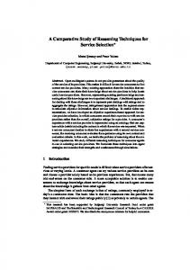
& Mees, 1995], which are linear combinations of arbitrary functions.1 As the condition for building models, broadly speaking, the more data points and the cleaner the data the better. However, conditions for building models are usually not so optimal, because time series available to us are usually contaminated by observational noise2 to a varying degree, and their length3 and numerical accuracy is also limited. That is, time series include the true phenomenon and noise. A simple example is given in Fig. 1. For building good models under such unfavorable conditions, we have to face three important problems [Nakamura, 2004]. Although these problems will be mentioned separately, they are strongly interconnected for building good models. The first is how to select basis functions which reflect the peculiarities of the time series as much as possible. We usually cannot know the best basis functions and the best combination of these basis functions before building models. The second is how to provide good estimates for the parameters in the basis functions. Estimated parameters may have a significant bias, when the noise included in the time series is significant relative to the nonlinearity. The third is how to find the model size so that the models can reflect the underlying system and so that the
Intensity
3
2
1
0
Fig. 1.
1
noise free data (true phenomenon) observed data (true phenomenon and observational noise)
0
20
40
60
Iteration
80
100
A simple example of noise free and noisy time series.
influences of noise included in the data are removed as much as possible. In this paper, we focus on this third problem. The question of what is an appropriate model size is an old one. To identify a satisfactory model size (we will write more details on models we adopt and model size in Sec. 2) when time series are contaminated by observational noise, information criteria are often applied [Mees, 1993]. A variety of information criteria have already been proposed, each with a different background. Information criteria were originally employed to investigate the influence of “observational noise” in modeling, however, it is expected that many systems in the real world are also perturbed by “dynamic noise”.4 There is, however, not much discussion concerning the influence of dynamic noise in modeling. Also, the practical formulae for the information criteria we use are derived on the assumptions that the fitting error (prediction error) is normally distributed and that the number of data used is large enough [Akaike, 1974; Schwarz, 1978; Rissanen, 1989, 2000; Judd & Mees, 1995]. Under the ideal conditions, any information criterion will work well enough and select the same model (or almost the same) as the best model.5 However, in practice, the assumptions do not always hold. As a result, the model selected as the best model will be influenced by information criteria we choose. Also, although applying information criteria has proven to be effective in modeling nonlinear dynamics [Judd & Mees, 1995, 1998; Small & Judd, 1998], all models we build from time series are lies [Mees, 2000]. That is, in practice there is no correct model. In such cases, it is clear that the quality of a model is more important than the number of parameters in the model. However, we consider that the minimum value of the information criterion yields the best model works well irrespective of correct models or not. For these reasons, we consider that it is both important and necessary to investigate the
We call these basis functions, although they need not actually be a basis. If the noise only affects the observation of the system, the noise is called “observational noise”. 3 Although it is sometimes possible to obtain very long data length, for example, in laboratory experiments, it is not always possible in the real world. Often the data length cannot increase easily. For example, the data length of annual sunspot numbers is around 300, which date from the year 1700. To obtain the only 1000 data point, we would need to wait for another 700 years! 4 When an output of a dynamical system becomes corrupted with noise or in other words, the system is perturbed by noise, and the value is used as the input to the system during the next iteration, the noise is called “dynamic noise” or “dynamical noise”. 5 We will give more details on how to consider and select the best model using information criteria in Sec. 2. 2
A Comparative Study of Information Criteria for Model Selection
adequacy and problems of using information criteria using known models in detail under practical conditions before applying information criteria in practice. In Sec. 2, we introduce the information criteria to be discussed in this paper. To demonstrate the performance of the information criteria impartially, we compare them under the same conditions. We then discuss their efficacy by comparing the performance and discuss some problems.
2. Information Criteria In this section, we describe pseudo-linear models which we adopt for building models, basic ideas of using information criteria and the backgrounds of the information criteria to be applied.
2.1. Pseudo-linear models Pseudo-linear models are a particularly convenient class of nonlinear models which are a generalization of linear models such as AR model and have been applied widely [Judd & Mees, 1995]. The models we adopt in this paper are all pseudo-linear models. These have the general form k % xt+1 = λi fi (vt ), i=1 vt = (xt−!1 , xt−!2 , . . . , xt−!d ) ∈ Rd ,
where x is scalar data, fi are some selection of nonlinear basis functions, ("1 , "2 , . . . , "d ) is a lag vector where the entries are positive integers and "j+1 > "j [Judd & Mees, 1998], λi are unknown parameters, d is the embedding dimension and k is the number of basis functions. Define, Vi = (fi (vt ), fi (vt+1 ), fi (vt+2 ), . . . , fi (vt+n ))T , i = 1, 2, . . . , k T y = (xt+1 , xt+2 , . . . , xt+n+1 ) λ = (λ1 , λ2 , . . . , λk )T , 6
2155
where T indicates transpose and n is the number of ˆ is chosen to minimize the sum data points. The λ ˆ where λ ˆ of squares of the fitting error e = y − V λ, is an estimate of λ. The attraction of pseudo-linear models is that the parameters are easily calculated, because the sum of squares of the fitting errors can be minimized efficiently by the least squares (LS) method using singular value decomposition or any of its many equivalents.6 Here, the model size refers to the number of basis functions, which is the same as the number of parameters of the model, because the only parameters used to fit the data are the linear weights [Nakamura et al., 2004]. In order to build “good” pseudo-linear models not all basis functions are suitable. We should use basis functions that can extract the peculiarities of the time series as much as possible. That is, the challenge of pseudo-linear models comes from the selection of fi , the basis functions.7 Clearly, the more fi the better the approximation of the data. However, time series available to us are usually contaminated by observational noise and so we do not want to over-fit the data, because our purpose is to build models that can reflect the underlying system and remove the influence of noise as much as possible. In the next section, we will discuss this problem.
2.2. Basic ideas of using information criteria To build models which meet our purpose it is important to decide on the model size.8 The model should not be fitted to the data too closely; this is called “over-fitting”. Conversely, if the model is not well fitted to the data, it is said “under-fitting”. In both the cases, the model often becomes unstable and also has difficulty in prediction. Figure 2 shows a rough sketch of the relationship between model size (number of parameters) and fitting error (prediction error) for a generic information criterion.
The maximum likelihood estimate (MLE) which corresponds to a normal probability distribution is the LS method. That is, we apply the LS method under the assumption that the fitting error is normally distributed, and the fitting error is used to calculate the information criteria. In practice, we usually apply the LS method as the MLE, even if the assumption does not hold, because of the elegant approximation derived from the assumption. In Sec. 4.2 we will discuss the LS method and show the reason why the fitting error is not normally distributed and the fitting errors are uncorrelated with the observational noise, even if the observational noise is Gaussian. 7 These models can be obtained by starting with a large dictionary of basis functions, which one hopes will be able to describe any likely nonlinearity; selecting a small subset; and, taking a linear combination of these to form a model. Selecting the optimal subset of basis functions is typically an NP-hard problem [Judd & Mees, 1995]. More details about selection methods are elsewhere [Nakamura et al., 2004]. 8 It is also important to generate and select good basis functions.
T. Nakamura et al.
Information Criterion
2156
Best model (Optimal model) Penalty for model size
Fitting errors
0
5
10
20
15
Model size (number of parameters) Fig. 2.
Information criterion as a function of model size.
As the figure shows, information criteria are used to find the model that best balances model error against model size so as to prevent over-fitting or under-fitting of the data. It is considered that the minimum of the information criterion corresponds to the best (optimal) model size and the smaller the value, the better the model [Akaike, 1974; Judd, 2003]. Another important reason for using information criteria is to avoid unnecessary increase in the model size. This can occur when a reconstructed model is an iterated form of a smaller model. We refer to this kind of model as nested or degenerate. A simple example is the following. Let the original model be xt = a1 xt−1 + a3 xt−3 ,
(1)
which has model size 2. This model can be rewritten as xt−1 = a1 xt−2 + a3 xt−4 .
(2)
Using expression (2) to replace the basis function (1/2)xt−1 , for example, in the original model gives 1 1 xt = a1 xt−1 + a1 xt−1 + a3 xt−3 2 2 1 1 = a1 xt−1 + a1 (a1 xt−2 + a3 xt−4 ) + a3 xt−3 2 2 1 1 1 = a1 xt−1 + a21 xt−2 + a3 xt−3 + a1 a3 xt−4 . 2 2 2 (3) Although model (3) is identical to the original model (1), its size is 4, which is larger than that of
the original model. If the data are noisy, any equation and the identities would no longer be satisfied at the original equation exactly for any time. Degenerate models are effective for reducing fitting error, because the formulae are some kind of a moving average filter. If such an operation is done continuously, the model size increases infinitely. Hence, it is important to remove the nesting effect and determine the smallest model size which can substantially model the system, because larger models are clearly over-fitting. For more details, see [Judd, 2003; Nakamura & Small, 2006]. Some information criteria have been proposed for these purposes. The most well-known information criterion is the Akaike Information Criterion [Akaike, 1974]. After his pioneering work, other criteria were proposed, such as the Schwarz Information Criterion [Schwarz, 1978], Description Length and Predictive Description Length [Rissanen, 1989], Rissanen’s Description Length modified by Judd and Mees [1995] and the Normalized Maximum Likelihood [Rissanen, 2000]. We briefly review the backgrounds of these information criteria. Here we note that the data x = x1 , x2 , . . . , xn are assumed to be a set of independent identically distributed (i.i.d) observations of a statistical model p(x|λ) with unknown parameters λ ∈ Rk (k is the model size, that is, the number of parameters). When x is given, p(x|λ) is called a likelihood of the ˆ be the maximodel given for parameters λ. Let λ mum likelihood estimate (MLE) of the parameter λ obtained from data x. The number of data points used is n and e is fitting error.
2.3. Akaike Information Criterion Akaike proposed measuring the goodness of fit of a statistical model using the amount of deviation of the “true” distribution from the predicted distribution of the model [Akaike, 1974], and evaluating this quantity using Kullback–Leibler information [Kullback & Leibler, 1951]. The Akaike Information Criterion (AIC) is defined as ˆ + 2k. AIC = −2 ln p(x|λ) In practice, under the assumption that the fitting error is normally distributed, the AIC formula is AIC(k) = n ln
eT e + 2k. n
(4)
A Comparative Study of Information Criteria for Model Selection
2.4. Schwarz Information Criterion Schwarz proposed an alternative approach to model order estimation [Schwarz, 1978]. It is called the “Schwarz Information Criterion” (SIC) [Judd & Mees, 1996] and is also known as the “Bayesian Information Criterion” (BIC) [Barron et al., 1998]. It is defined as ˆ + k ln n. SIC = −2 ln p(x|λ)
Under the assumption that the fitting error is normally distributed, the SIC formula is SIC(k) = n ln
eT e + k ln n. n
(5)
2.5. Description length Rissanen proposed the description length principle [Rissanen, 1989], which seeks to minimize the number of bits needed to describe the data using available models when the system is unknown. That is, the best model is the one that describes the data with the shortest description length.9 It is called the minimum description length (MDL) principle. There are two procedures to estimate description length. One is two-part code and the other is onepart code.
A convenient, although sub-optimal, way to reconstruct the data would be to use the model and its parameters, including initial data, and to then correct the model’s output by adding in the fitting errors. This gives a so-called two-part code: the model and its error vector can be used to reconstruct the data. Judd and Mees showed that the description length DLγ can be approximated by ' & ' & eT e 1 n − 1 ln + (k + 1) + ln γ DLγ (k) = 2 n 2 k % i=1
ln δi
under the assumption that the fitting error is normally distributed [Judd & Mees, 1995]. It should be noted that in practice γ typically takes values between 1 and 32, where γ is the exponent in a floating point representation of the parameters scaled relative to some fixed amount [Judd & Mees, 1995]. A value γ = 1 gives larger models and a value γ = 32 gives smaller models. However, there is no reliable theory and knowledge to indicate the correct value of γ. We investigate the influence of different values of γ in this paper.
2.5.2. Predictive Description Length as a one-part code Quite a different approach to description length is from the viewpoint of “predictive coding” [Rissanen, 1989]. This gives a one-part code: it requires building a model iteratively as the transmitted data is received (that is, it encodes the data x1 x2 . . . xn one by one). Since the model used here can be regarded as a function of λ, it will be written as f (x, λ) temporarily. Using the whole of the data xt−1 = xt−1 up to the time t − 1, λt−1 is estimated x1 , . . . , ( 2 as min t−1 i=1 #xi − f (xi−1 , λ)# . Using λt−1 , the fitting error of the model at time t, et = xt − f (xt−1 , λt−1 )
2.5.1. Description length as a two-part code
−
2157
(6)
is calculated, then we obtain the Predictive Description Length (PDL), n % e2t . (7) PDL = i=1
In practice, under the assumption that the fitting error is normally distributed, the parameter λ is estimated by the LS method, and for time t smaller than the model size the raw data is sent (that is, et = xt ) because it is impossible to estimate the parameters.
2.6. Normalized Maximum Likelihood Recently, Rissanen proposed a new information criterion, whose form of description length is based on
9 Minimum Message Length (MML) proposed by Wallance and Freeman [1987] has similar motivation to Description Length, because minimum encoding inference is used in the criteria. The different principles are: MML is concerned with models. That is, the end result of MML inductive inference is a model with specified parameter values. MDL has an additional emphasis on “data modeling”, the prediction of new data using model classes. Hence, if MDL is used for prediction of new data, no selection of models or parameter estimates are necessarily needed in the message. See more details on MML and differences and similarities between MML and MDL elsewhere [Oliver & Hand, 1994; Oliver & Baxter, 1994; Baxter & Oliver, 1994; Lantermanm, 2001].
2158
T. Nakamura et al.
the Normalized Maximum Likelihood (NML) coding scheme [Rissanen, 2000]. When just a set of parameters is given, we have to retain the possibility that any (or all) data may have occurred. However, if we know the fact that the parameters were estimated using maximum likelihood, we can restrict the possible data to only those data giving the same parameter estimates. NML represents a measure which ˆ ˆ T (V λ)/n. ˆ = (V λ) Under reflects the idea. Let R the assumption that the fitting error is normally distributed, Rissanen derived, asymptotically, the formula ' & n − k eT e k ˆ − ln Γ n − k NML(k) = ln + ln R 2 n 2 2 & ' k − ln k, (8) − ln Γ 2 where Γ is the Gamma function.
3. Investigation of the Information Criteria We investigate a number of proposed information criteria, and the adequacy of the idea that the minimum value of the information criterion yields the best model. To investigate the behavior of information criteria we use five models where three are polynomial models (linear auto-regressive (AR), nonlinear AR and nonlinear moving average (MA)) and the others are models using basis functions (a model of the Lorenz equations using ellipsoid basis functions (EBFs) and a model of the annual sunspot numbers using radial basis functions (RBFs)). We also consider a linear AR model and a model using RBFs perturbed by dynamic noise. We treat these models as the correct models. We add all basis functions included in each correct model into a larger dictionary. Here, we note that the “correct model” means that only all basis functions included in the correct model are selected. Also, when a model has the smallest value of an information criterion among many models, we call the model the “best model”. We investigate what is the best model even if the correct model belongs to the chosen model class. We expect that the information criteria should be 10
a minimum when the model built is the correct model (that is, the best model is the correct model). Constructing pseudo-linear models is NP-hard, because the optimal subset of basis functions has to be selected from a large dictionary of basis functions [Judd & Mees, 1995]. Usually a selection method is applied for selection of the subset. Some methods have been proposed [Chen et al., 1991; Judd & Mees, 1995; Nakamura et al., 2003, 2004]. One of the difficulties is there are local minima, and it is difficult to find a global best model. Hence, to avoid any influence of selection methods and to find truly the best model, we calculate all possible combinations of basis functions from the dictionary. We add four different levels of Gaussian observational noise to all models, namely 10 dB, 20 dB, 40 dB and 60 dB.10 We use data sets of length 1000, 10 000 and 100 000. We also check the distribution of fitting errors in the correct models when the noise level is 40 dB and the number of data points used is 100 000.11
3.1. A linear AR model The following model appears in [Small & Judd, 1999]. xt = A0 + A1 xt−1 + A6 xt−6 + ηt , yt = xt + &t , where A0 = 2.945206, A1 = 0.300739 and A6 = 0.202056, ηt is Gaussian dynamic noise and &t is Gaussian observational noise. We use yt as observational data and will use time delay linear polynomial models. Choosing a lag = 9 gives 10 candidate basis functions in the dictionary. These are the constant function and xt−1 , xt−2 , . . . , xt−9 . Using the dictionary we can build a model xt−1 = A0 + A1 xt−2 + A6 xt−7 from which we can build the degenerate models. Table 1 shows the best value of each information criterion in each model size. In most cases, the correct model is selected as the best model by DL1,4,8,32 , NML, PDL and SIC, even when the noise level is high. However, AIC cannot select the correct model as the best model in most cases. Also, although we can build the degenerate models from the dictionary, the size of the model selected as the
We will express the noise level in terms of the approximate signal to noise ratio (SNR), measured in decibels. To determine the standard deviation of the Gaussian for each noise level, 10 000 data points are used. 11 The reason we adopt these values is that a large number of data points is always better for estimating statistics and if the noise level is very large or very small, it is not easy to discriminate between the dynamics and the noise. From our experience, when the noise level is 40 dB, the parameters estimated using the time series are usually close to the correct values.
A Comparative Study of Information Criteria for Model Selection
2159
◦
Table 1. The result in each information criterion when the model used is a linear AR model. The , " and × indicate the model selected as the best model. The indicates that the correct model is selected when an information criterion is the smallest (that is, the best model from the viewpoint of information criteria is the correct model). The " indicates that the correct model is selected in the correct model size, however, the information criterion is not the smallest (that is, there are other models of another size whose information criterion is smaller than that of the correct model). The × indicates that the wrong model is selected in the correct model size (that is, we cannot select the correct model in this case.). The first entry in parentheses is the amount by which the size of the best model exceeds that of the correct model. The second entry is the error in the information criterion of the best model from that of the correct model. The error is expressed as a percentage of the absolute value of the value of the correct model minus the value of best model divided by the value of best model.
◦
SNR
Number of Data Points
DL1
DL4
DL8
DL32
NML
PDL
AIC
SIC
!
!
!
!
!
!
" (+1, 3.523%)
" (+1, 0.768%)
" (+1, 0.14%)
!
!
!
" (+1, 0.009%)
!
" (+5, 1.10%)
" (+1, 0.57%)
100 000
!
!
!
!
!
!
" (+4, 0.14%)
" (+1, 0.003%)
1000
!
!
!
!
!
!
" (+1, 3.78%)
!
10 000
!
!
!
!
!
!
" (+2, 1.53%)
!
100 000
!
!
!
!
!
!
" (+1, 0.02%)
!
1000
!
!
!
!
!
!
" (+1, 2.383%)
!
10 000
!
!
!
!
!
!
" (+2, 1.80%)
!
100 000
!
!
!
!
!
!
!
!
1000
!
!
!
!
!
!
" (+1, 1.29%)
!
10 000
!
!
!
!
!
!
" (+2, 1.78%)
!
100 000
!
!
!
!
!
!
!
!
1000 10 dB
20 dB
40 dB
60 dB
10 000
best model is the same as that of the correct model in most cases. That is, we can avoid unnecessary increase in the model size. Figure 3 shows the distribution of the fitting error when the model is correct. The histogram is obtained from the fitting errors and the solid line is a theoretical Gaussian with the same standard deviation as that of the fitting errors. Notice that the fitting error in panel (b) is shown on a logarithmic scale so that discrepancy can be easily examined. As Figs. 3(a) and 3(b) show, the distribution of the fitting error in the correct model is almost the same as the normal distribution, which is the assumption used to derive the information criteria.
3.2. A nonlinear AR model The Henon map [Henon, 1976] is described by the equations xt = A0 + A1 xt−2 + A2 x2t−1 , yt = xt + &t , where A0 = 1.0, A1 = 0.3 and A2 = −1.4 and &t is Gaussian observational noise. We use yt as observational data and will use time delay linear polynomial models. Choosing a lag = 2 and a degree = 3 gives 10 candidate basis functions in the dictionary, these are the constant function, xt−1 , xt−2 , x2t−1 , x2t−2 , xt−1 xt−2 , x3t−1 , x3t−2 , x2t−1 xt−2 and xt−1 x2t−2 .
2160
T. Nakamura et al. 8000 7000
10
4
10
3
10
2
10
1
10
0
5000
Frequency
Frequency
6000
4000 3000 2000 1000 0 −4
−2
0
2
4
Class (a)
−4
−2
0
2
4
Class (b)
Fig. 3. The distribution of the fitting error when the model is the correct linear AR model, SNR = 40 dB and n = 100 000, shown with a (a) standard scale and (b) logarithmic scale. The solid line is a theoretical Gaussian with mean and standard deviation the same as the fitting error of the correct model.
Table 2 shows the best value of each information criterion in each model size. When the noise level is high, although the correct model is selected in the correct model size, it is not selected as the best model in most cases. When the noise level is low, the correct model is selected as the best model in most cases. However, when SNR = 40 dB and the number of data points is 100 000, the correct model is not selected as the best model except by PDL. Furthermore, the typical model size chosen was much larger than the correct model size. Figure 4 shows the distribution of the fitting errors when the model is the correct model. Figures 4(a) and 4(b) show clearly that the distribution of the fitting error in the correct model is not normally distributed, which is not consistent with the assumption used in deriving the information criteria. This implies that there are some kind of systematic errors. When SNR = 40 dB and n = 1000 or 10 000 the best model is correct in most cases. However, when n = 100 000 the size of the best model is 8, which is much larger than the correct model size 3. A possible explanation for this is that when n = 1000 or 10 000 and SNR = 40 dB the influence of the systematic error is less significant than when n = 100 000. Hence, when a smaller number
of data points is used, the correct model is obtained as the best model, although there are still some systematic errors. However, as the number of data points used increases, the influence of systematic error becomes more significant. Since this influence cannot be bypassed, the size of the model selected as the best model will be larger than that of the correct model in order to reduce the influence of systematic error. To investigate the influence of systematic error in more detail, we increase basis functions in the dictionary. Choosing lag = 3 and degree = 3 gives 20 candidate basis functions in the dictionary. Using the dictionary we can build a model xt−1 = A0 + A1 xt−3 + A2 x2t−2 from which we can build the degenerate models. Since there are more combinations than lag = 2 and degree = 3 and it takes a long time to calculate PDL, we investigate using only 1000 data points. The results are presented in Table 3. The correct model is not the best model in all cases except for PDL, even when the noise level is low and the number of data points used is not many. In the previous example, the correct model is selected as the best model when the noise level is low and the number of data points used is small. However, this is not the case in this example. Furthermore, the size of
2161
60 dB
40 dB
20 dB
10 dB
SNR " (+2, 4.42%) " (+5, 6.19%) " (+7, 5.87%) " (+2, 1.13%)
" (+2, 4.72%)
" (+5, 6.26%)
" (+7, 5.88%)
" (+2, 1.28%)
10 000
100 000
1000
! !
! !
1000 10 000 100 000 !
" (+5, 0.02%)
" (+5, 0.022%)
100 000
!
!
!
!
10 000
!
" (+4, 1.99%)
" (+4, 1.99%)
100 000
1000
" (+3, 2.21%)
" (+4, 2.23%)
10 000
1000
DL4
DL1
Number of Data Points
!
!
!
" (+5, 0.019%)
!
!
" (+4, 1.99%)
" (+3, 2.20%)
" (+2, 1.05%)
" (+7, 5.86%)
" (+4, 6.15%)
" (+2, 4.27%)
DL8
!
!
!
" (+5, 0.018%)
!
!
" (+4, 1.98%)
" (+3, 2.17%)
" (+2, 0.90%)
" (+7, 5.85%)
" (+4, 6.08%)
" (+2, 3.96%)
DL32
!
!
!
" (+5, 0.011%)
!
!
" (+4, 0.54%)
" (+4, 0.73%)
" (+3, 0.60%)
" (+7, 0.82%)
" (+6, 1.11%)
" (+4, 1.22%)
NML
!
!
!
!
!
!
" (+5, 7.35%)
" (+4, 7.55%)
!
" (+7, 0.34%)
" (+4, 9.48%)
" (+4, 7.35%)
PDL
!
!
!
" (+5, 0.025%)
" (+6, 0.03%)
!
" (+3, 0.01%)
" (+6, 0.06%)
!
!
" (+1, 0.05%)
!
" (+4, 1.07%)
" (+4, 2.28%)
" (+3, 1.29%)
" (+7, 1.65%)
" (+6, 6.35%)
" (+3, 5.04%)
SIC
" (+5, 2.01%)
" (+5, 2.35%)
" (+3, 1.63%)
" (+7, 1.66%)
" (+7, 6.61%)
" (+7, 6.30%)
AIC
Table 2. The result in each information criterion when the model used is a nonlinear AR model (lag: 2, degree: 3). For the explanation of notations and values used in this table, see Table 1.
2162
T. Nakamura et al.
14000 12000
10
4
10
3
10
2
10
1
10
0
Frequency
Frequency
10000 8000 6000 4000 2000 0 −0.1
−0.05
0
0.05
0.1
−0.1
−0.05
0
Class (a)
0.05
0.1
Class (b)
Fig. 4. The distribution of the fitting error when the model is the correct nonlinear AR model, SNR = 40 dB and n = 100 000. (b) The graph is shown with a logarithmic scale. The solid line is a theoretical Gaussian with mean and standard deviation the same as the fitting error of the correct model.
the best model is much larger than that of the correct model. We investigate this phenomenon. The formula of the best model selected by some information criteria when SNR = 60 dB is xt = 0.7873 − 0.4188xt−1 + 0.3001xt−2
− 0.0638xt−3 − 0.7685x2t−1 + 0.2975x2t−2 − 0.1894xt−1 xt−3 + 0.8841xt−1 x2t−2 .
This is, in fact, a degenerate approximation to the correct model. We can find such degenerate approximations of size 6 when the noise level is 10 dB, sizes 6 and 8 when the noise level is 20 dB, and sizes 6, 8 and 11 when the noise levels are 40 dB and 60 dB. Furthermore, these degenerate models are selected as the best models in most cases. See the decomposition and more discussions about the model degeneracy elsewhere [Judd 2003; Nakamura, 2004; Nakamura & Small, 2006]. It should be noted that the selected model of size 3 under the same condition (that is, SNR = 60 dB and the number of data points is 1000) is xt = 0.9999 + 0.3001xt−2 − 1.4000x2t−1 . 12
Although the model is almost identical to the actual system model of the Henon map, the model of size 3 is not selected as the best model, which is a significant problem. As mentioned in Sec. 2.2, one of the important reasons for using information criteria is to avoid unnecessary increases in model size. In this simple example, no information criterion, besides PDL, works well.
3.3. A nonlinear MA model A nonlinear MA model is given xt = A1 µt−1 + A2 µ2t−1 + A3 µ3t−1 + A4 µ2t−1 µt−2 , yt = µt + &t , zt = xt + ξt , where the input signal µt is uniform random on [0, 1], A1 = 3.0, A2 = 2.0, A3 = 5.0 and A4 = 4.0, and &t and ξt are observational noise.12 We use yt and zt as observational data and will use time delay linear polynomial models. Choosing lag = 2 and degree = 3 gives 10 candidate basis functions in the dictionary. Table 4 shows the best value of each information criterion in each model size. When SNR = 10 dB and 20 dB, the correct model is not
In this example, two different observational noises are added to the input and output signals. The noise levels in each signal differ in amplitude in order to ensure the same decibel value for each signal.
2163
" (+4, 9.53%) " (+5, 4.64%) " (+5, 1.84%) " (+5, 1.01%)
" (+7, 10.17%) " (+5, 5.01%) " (+5, 2.01%) " (+5, 1.11%)
10 dB
20 dB
40 dB " (+5, 0.96%)
" (+5, 1.75%)
" (+5, 4.45%)
" (+4, 9.20%)
DL8
" (+3, 0.78%)
" (+5, 1.59%)
" (+5, 4.08%)
" (+4, 8.53%)
DL32
" (+5, 0.88%)
" (+5, 1.35%)
" (+5, 2.28%)
" (+9, 3.00%)
NML
" (+13, 7.08%) " (+11, 2.94%) " (+9, 1.89%)
! !
" (+13, 14.0%)
AIC
" (+3, 7.77%)
" (+9, 21.29%)
PDL
" (+5, 1.65%)
" (+5, 2.56%)
" (+9, 5.62%)
" (+9, 11.53%)
SIC
60 dB
40 dB
20 dB
10 dB
SNR × × × " (−1, 0.14%) " (+1, 0.002%) " (+1, 0.003%) ! ! ! ! ! !
× × × " (−2, 0.10%) " (+1, 0.007%) " (+1, 0.007%) ! ! ! ! ! !
10 000
100 000
10 000
100 000
1000
10 000
100 000
1000
1000
1000 10 000 100 000
DL4
DL1
Number of Data Points
!
!
!
!
!
!
" (+1, 0.0002%)
" (+1, 0.0002%)
" (−1, 0.16%)
× × ×
DL8
!
!
!
!
!
!
!
!
!
!
!
!
" (+1, 0.008%)
" (+1, 0.008%)
! " (+1, 0.004%)
" (−1, 0.011%)
× × ×
NML
" (−1, 0.21%)
× × ×
DL32
!
" (−1, 14.44%)
" (−2, 45.97%)
!
" (−1, 11.61%)
" (−2, 45.05%)
!
!
!
" (+1, 0.001%)
!
!
" (+6, 0.021%)
!
!
!
!
!
!
!
" (+1, 0.02%)
" (+1, 0.02%)
!
! " (+1, 0.030%)
× × ×
SIC × × ×
AIC
" (−1, 0.0002%)
" (−1, 0.006%)
× × ×
PDL
Table 4. The result in each information criterion when the model used is a nonlinear MA model (lag: 2, degree: 3). For the explanation of notations and values used in this table, see Table 1.
60 dB
1000
DL4
SNR
DL1
Number of Data Points
Table 3. The result in each information criterion when the model used is a nonlinear AR model (lag: 3, degree: 3). For the explanation of notations and values used in this table, see Table 1.
2164
T. Nakamura et al.
selected as the best model in most cases. However, when SNR = 40 dB and 60 dB, the correct model is selected as the best model in most cases except PDL. We investigate why PDL does not work well. When SNR = 40 dB and the n = 1000, the basis functions selected are µ2t−1 and µ2t−1 µt−2 . When SNR = 60 dB and n = 1000, the basis functions selected are µ2t−1 and µt−1 µt−2 . When SNR = 40 dB or 60 dB and n = 10 000, the basis functions selected are µt−1 , µ3t−1 and µ2t−1 µt−2 . From this, we expect that there is no significant difference between the basis functions selected, and some basis functions are in the correct model because the input signal µt is in [0, 1]. For example, when µt−1 = 0.01, µ2t−1 = 0.0001 and µ3t−1 = 0.000001. There are difference in these values, but these are actually “nearly” 0. Hence, µt−1 or µ3t−1 would compensate for µ2t−1 when SNR = 40 dB or 60 dB and n = 10 000. Since this problem does not occur with other information criteria, this might be a characteristic of PDL. This demonstrates a serious disadvantage of PDL. Figure 5 shows the distribution of the fitting error when the model is correct. As Figs. 5(a) and 5(b) show clearly, the distribution of the fitting error in the correct model is not normal, which contradicts the assumption used to derive the
information criteria. This implies that there are systematic errors.
3.4. A model of the Lorenz equations using EBFs The training set is generated from the Lorenz equations [Lorenz, 1963]: dy = −y − xz + rx, dτ
dx = −σ(x − y), dτ
dz = xy − Bz, dτ with σ = 10.0, r = 24.73, B = 8/3, by using an adaptive Runge–Kutta method with sampling interval 0.1. We use the x component of the Lorenz equations as the training set. The data is embedded using a uniform embedding Xt−1 = (xt−1 , xt−3 , xt−5 ) in three dimensions for predicting xt . A model is built using the “behavior criterion” [Kilminster, 2003]. The model has 7 EBFs, where a EBF has different radius unlike a RBF, and we use it as the correct model. We use a free-run time series of the model as observational data. Figure 6 shows the training time series of the Lorenz equations, a free-run of the model, and their
12000 4
10
8000
Frequency
Frequency
10000
6000
3
10
2
10
4000 1
10
2000
0 −0.4
0
10 −0.3
−0.2
−0.1
0
0.1
0.2
0.3
0.4
−0.4
−0.3
−0.2
−0.1
0
Class
Class
(a)
(b)
0.1
0.2
0.3
0.4
Fig. 5. The distribution of fitting error when the model is the correct nonlinear MA model, SNR = 40 dB and n = 100 000. (b) The graph is shown with a logarithmic scale. The solid line is a theoretical Gaussian with mean and standard deviation the same as the fitting error of the correct model.
A Comparative Study of Information Criteria for Model Selection
20
Training data of Lorenz equations
20
Free–run data of the EBF model
10
x(t)
x(t)
10 0 −10
0 −10
−20
0
100
200
300
400
−20
500
0
100
Iteration
20
400
500
Reconstructed attractor using free–run data
10
x(t2)
10
x(t2)
300
(b)
Reconstructed attractor using training data
0
−10
−20 −20
200
Iteration
(a)
20
2165
0
−10
−10
0
10
20
x(t) (c)
−20 −20
−10
0
10
20
x(t) (d)
Fig. 6. Time series of training data of the Lorenz equations and a free-run of the model, along with reconstructed attractor of these time series.
corresponding attractors. These are very similar to the original time series of the Lorenz equations.13 In the previous examples, increasing lag and degree can generate other basis functions to add into a dictionary. This is possible because the models are all polynomial. However, as the basis function used is EBF, we use the following idea. We first generate other basis functions by randomizing all parameters in the 7 EBFs in the correct model, then, we choose a model size of 12 and thus take another 5 EBFs from them. Table 5 shows the best value of each information criterion in each model size. When 13
SNR = 10 dB and 20 dB, the correct model is never selected. These noise levels are far too large for modeling. When SNR = 40 dB and 60 dB, the correct model is selected as the best model in some cases. However, AIC never selects the correct model as the best model. Figure 7 shows the distribution of the fitting error when the model is the correct model. As Figs. 7(a) and 7(b) clearly show, the distribution of the fitting error in the correct model is not normal, which contradicts the assumption used to derive the information criteria. This implies that there are systematic errors.
We use a term of “similar” not from the viewpoint of a dynamical points but visual inspection. Further investigations are necessary to indicate that the dynamics of the model we use is the same as that of the Lorenz equations. However, it is enough for us to use a model in this study, if the model generates stable trajectories.
2166
60 dB
40 dB
× × ×
× × ×
1000 10 000 100 000
20 dB
! !
10 000
100 000 !
!
!
" (+2, 0.011%)
" (+2, 0.013%)
100 000
!
!
" (+1, 0.003%)
10 000
1000
" (+1, 0.02%)
" (+1, 0.10%)
1000
× × ×
× × ×
DL4
DL1
1000 10 000 100 000
Number of Data Points
10 dB
SNR
!
!
!
" (+2, 0.010%)
!
!
× × ×
× × ×
DL8
!
!
!
" (+2, 0.009%)
!
!
× × ×
× × ×
DL32
!
!
!
" (+2, 0.002%)
!
!
× × ×
× × ×
NML
!
!
!
" (+1, 22.33%)
×
×
× × ×
× × ×
PDL
" (+2, 0.012%) ! ! !
" (+1, 0.057%) " (+2, 0.004%) " (+1, 0.0004%)
!
!
× × ×
× × ×
SIC
" (+4, 0.019%)
" (+1, 0.009%)
" (+1, 0.043%)
× × ×
× × ×
AIC
Table 5. The result in each information criterion when the model used is an EBF model of the Lorenz equations. For the explanation of notations and values used in this table, see Table 1.
A Comparative Study of Information Criteria for Model Selection
2167
12000 10
4
10
3
10
2
10
1
10
0
10000
Frequency
Frequency
8000
6000
4000
2000
0 −1
−0.5
0
0.5
−1
1
−0.5
0
Class
0.5
1
Class
(a)
(b)
The period 1700–2000 of the annual sunspot numbers is first used to build the correct model. We transform the raw annual sunspot √ numbers st using the nonlinear function xt = 2 st + 1 − 1 [Tong, 1990]. The data is embedded using nonuniform embedding Xt−1 = (xt−1 , xt−2 , xt−4 , xt−8 , xt−10 ) in five dimensions for predicting xt [Kilminster, 2003], where RBFs are used. Using the period 1700–2000 of the annual sunspot numbers, a model is built using two linear (t − 1 and t − 2) and three RBFs using the “behavior criterion” [Kilminster, 2003], and we use it as the correct model. We use a free-run time series of the model as observational data. Figure 8 shows the original annual sunspot numbers and the free-run time series of the model, which is very similar to the original time series of the annual sunspot numbers. The model appears to be a reasonable proxy for the true physical system and so we use the model to generate a representative time series with which to test the information criteria. As is the case with the previous section, to make a dictionary, other RBFs are first generated and we choose a model size of 10 and thus take another five RBFs from them.
200 150 100 50 0 1700
1800
Year
1900
2000
200
300
(a) 200 150
x(t)
3.5. A model of the annual sunspot numbers using RBFs
Annual sunspot number
Fig. 7. The distribution of the fitting error when the model is the correct EBF model, SNR = 40 dB and n = 100 000. (b) The graph is shown with a logarithmic scale. The solid line is a theoretical Gaussian with mean and standard deviation the same as the fitting error of the correct model.
100 50 0 0
100
Iteration (b)
Fig. 8. Time series of (a) actual annual sunspot numbers and (b) a free-run of the model.
Table 6 shows the best value of each information criterion in each model size. When SNR = 10 dB and 20 dB, the correct model is not selected as the best model in most cases. When SNR = 40 dB
2168
60 dB
40 dB
20 dB
10 dB
SNR
!
" (+5, 0.092%)
" (+1, 0.001%) " (+5, 0.105%)
10 000
100 000
!
100 000
!
1000 !
!
100 000
10 000
!
10 000
!
!
!
!
!
!
×
×
1000
!
× × ×
× × ×
1000 10 000 100 000
1000
DL4
DL1
Number of Data Points
!
!
!
!
!
!
" (+5, 0.086%)
!
×
× × ×
DL8
!
!
!
!
!
!
" (+3, 0.076%)
!
×
× × ×
DL32
!
!
!
!
!
!
" (+5, 0.011%)
!
" (−1, 0.046%)
× × ×
NML
×
" (+2, 0.003%)
" (+1, 0.003%)
!
× ×
" (+1, 0.002%)
×
" (+1, 0.005%)
!
× ×
" (+5, 0.036%)
" (+3, 0.09%)
× ×
!
× × ×
AIC
×
× × ×
PDL
!
!
!
!
!
!
" (+5, 0.025%)
!
!
× × ×
SIC
Table 6. The result in each information criterion when the model used is a RBF model of the annual sunspot numbers. For the explanation of notations and values used in this table, see Table 1.
A Comparative Study of Information Criteria for Model Selection
and 60 dB, the correct model is selected as the best model in most cases except AIC and PDL. It should be noted that PDL does not work in all SNR and data points. When SNR = 20 dB and n = 1000, DL1,4,8,32 cannot find the correct model, although
2169
AIC, SIC and NML find the correct model. Since the new RBFs included in the dictionary are generated from three RBFs of the correct model, there is significant collinearity among these basis vectors. As DLγ takes into account the relative accuracy
7000
10
4
10
3
10
2
10
1
10
0
5000
Frequency
Frequency
6000
4000 3000 2000 1000 0 −8
−6
−4
−2
0
2
4
6
−8
8
−6
−4
−2
0
2
4
6
8
Class
Class (a)
(b)
Fig. 9. The distribution of the fitting error when the model is the correct RBF model, SNR = 40 dB and n = 100 000. (b) The graph is shown with a logarithmic scale.
7000
10
4
10
3
10
2
10
1
10
0
6000
Frequency
Frequency
5000 4000 3000 2000 1000 0 −8
−6
−4
−2
0
Class (a)
2
4
6
8
−8
−6
−4
−2
0
2
4
6
8
Class (b)
Fig. 10. The distribution of the fitting error when the model is the correct RBF model, SNR = 20 dB and n = 100 000. (b) The graph is shown with a logarithmic scale. The solid line is a theoretical Gaussian with mean and standard deviation the same as the fitting error of the correct model.
2170
T. Nakamura et al.
of different basis functions, the correct model will probably not be selected. When we compare the DLγ values of the correct models and the models selected, there are no significant differences between them. Figure 9 shows the distribution of the fitting error when the model is the correct model. As Figs. 9(a) and 9(b) show, the distribution of the fitting error in the correct model is normal, which agrees with the assumption used to derive the information criterion. When SNR = 20 dB and n = 100 000, the correct model is not selected as the best model, although it is selected as the best model when n = 10 000. We have checked the distribution of the fitting error in this case. As Fig. 10 shows, the distribution is almost normal, although it is slightly flattened and broadened. The reason why the correct model is not selected as the best model when n = 100 000 is probably because of the large noise influence. It indicates that even if the fitting error is almost normally distributed, if observational noise is large, then the correct model is not always selected.
4. Discussion Pseudo-linear models must be tuned via parameter estimation, and the least squares (LS) method is applied for this estimation. Fitting error is calculated using the models, and then information criteria are calculated using the fitting error. That is, as they are interconnected, calculation of fitting error is important. Hence, we investigate the nature of the fitting error and the LS method. We first compare the standard deviation (SD) of the observational noise added and the fitting error in each model. Secondly, we investigate the LS method in more detail.
4.1. SD of observational noise and fitting error Table 7 shows the standard deviation (SD) of Gaussian observational noise added and fitting errors in each model. The SD in each example is always larger than that of the observation noise. Especially, the difference when the models are linear AR model and the model of the annual sunspot numbers using RBFs are very significant. In both the models, the systems are perturbed by dynamic noise. For the linear AR model the SD of the Gaussian dynamic noise is 1.0, and for the model of the annual sunspot numbers using RBFs it is 1.52200369. Hence, it is reasonable that the SD values of these fitting errors are much larger than those of the observational noises added. However, in the other models; the nonlinear AR model, nonlinear MA model and model of the Lorenz equations using EBFs, the reason why the SD of these fitting errors are larger than those of the observational noise is probably due to systematic errors. Furthermore, as shown in previous sections, in all nonlinear models used except the model of the annual sunspot numbers using RBFs, the distribution of the fitting error in the correct model is not normal. The difference between these nonlinear models and the model of the annual sunspot numbers using RBFs is the presence of dynamic noise. We briefly consider this phenomenon. The SD of 40 dB observational noise for the RBFs model is 0.0555096662 and that of dynamic noise is 1.52200369, which is much larger than that of the observational noise. As mentioned above, although we consider that there are systematic errors in the other nonlinear models, we also expect that there probably exists systematic errors in the RBFs model, because the model is also nonlinear. Table 7 shows that the SD of fitting errors in the other nonlinear models are at most around 2.5 times as that of
Table 7. Comparison of the Standard Deviation (SD) of Gaussian observational noise added and fitting errors when SNR = 40 dB and n = 100 000, where the linear AR model and the model using RBFs have dynamic noise. Model Linear AR model Nonlinear AR model Nonlinear MA model A model using EBFs A model using RBFs
SD of Observational Noise
SD of Fitting Errors
0.0108603133 0.0072366961 0.0346424565 0.0778919619 0.0555096662
1.0056095860 0.0172907028 0.0531027313 0.1667765346 1.5235564852
A Comparative Study of Information Criteria for Model Selection
observational noise. However, the SD of dynamics noise is around 27 times as that of observational noise. From this, even if there are systematic errors in the RBFs model, we expect that the SD is smaller than that of dynamic noise. That is, the influence to the fitting error due to observational noise would be smaller than dynamic noise. As a result, we consider that the fitting error of the RBFs model would be normally distributed.
4.2. The relationship between fitting error and the LS method In previous examples, we found that the fitting error is not always normally distributed, although the observational noise is Gaussian. It is a significant problem, because it contradicts the assumption used to derive the information criteria. As a result, the best model size tends to be larger. In order to take advantage of information criteria effectively and to the fullest, we should attempt to remove systematic errors and now consider a method of doing so (see [Nakamura & Small, 2006] for a thorough description). We consider that the problem is due to the commonly used LS method, where the LS method is used to estimate parameters. We first note that we have a model xt+1 = f (xt , λ), xt ∈ R, where λ ∈ Rk is the parameter vector, and a time series of observations st contaminated by observational noise &t , that is, st = xt + &t . A commonly used LS method is min λ
n−1 % t=1
#st+1 − f (st , λ)#2 ,
(9)
where n is the number of data points. This is a maximum likelihood method which makes the assumption that the noise is Gaussian and independent for each observation st . For nonlinear models the LS does not provide good estimates of the parameters, which can have significant bias, especially when the noise is not small. This usage of the method effectively assumes noise only affects the “response” variables st+1 and not the “regressor” variables st , which is clearly false. This bias can be attributed to the so-called “error in variables” problem [McSharry & Smith, 1999]. In other words, even when the assumption holds and the noise is white, the LS is biased in the presence of observational noise. White observational noise at the output becomes colored regression noise in the regression equation which the LS cannot handle.
2171
The following usage is clearly better, min λ
n−1 % t=1
#st+1 − f (xt , λ)#2 ,
(10)
where xt is the true state (that is, noise free) at time t. However, of course we cannot know xt and hence in Eq. (9) st is used as a proxy for xt . We expect that Eq. (10) would be able to improve the information criteria estimation. As a demonstration, we investigate the nonlinear AR model (the Henon map) used in Sec. 3.2. As Table 3 shows, when only the noisy data and a dictionary of 20 candidate basis functions are used, all information criteria except PDL do not work even when the noise level is low. That is, the correct model is not selected as the best model, and a degenerate model is usually selected as the best model. Here, we use the previous true state (noise free) data and the current noisy datum to investigate the performance of the optimization problem (10), with noise levels 20 dB, 40 dB and 60 dB and number of data points 1000, where the best models selected were the degenerate models in these conditions. We again calculate all possible combinations to obtain the truly best model and take the best model in each information criterion. As Table 8 shows, all information criteria except AIC select the correct model as the best model at all noise levels. That is, the degenerate models, which were selected as the best models when using only the noisy data, are not selected as the best models. Actually, the models of size 6, 8 and 11 at all noise levels are no longer degenerate, although the models were mostly degenerate when using only the noisy data, that is, when using expression (9). The size of the best model selected by AIC at all noise levels is just one larger than that of the correct model. This is much better than when using only the noisy data. See Table 3. We also investigate the fitting errors and observational noise added, which is Gaussian, when the noise level is 40 dB and the number of data points is 1000 (see Fig. 11). Panel (a) shows that the fitting errors using Eq. (9) and the observational noise added are uncorrelated. This seems to indicate that there is no connection between the fitting error and the observational noise. Panel (b) shows that the fitting errors using Eq. (10) and the observational noise added are almost identical.
2172
T. Nakamura et al. Table 8. The result in each information criterion when the model used is a nonlinear AR model (lag: 3, degree: 3), where the previous true state (noise free) data and the current noisy datum are used. For the explanation of notations and values used in this table, see Table 1.
SNR
Number of Data Points
20 dB 40 dB
1000
60 dB
DL1
DL4
DL8
DL32
NML
PDL
AIC
SIC
!
!
!
!
!
!
" (+1, 0.011%)
!
!
!
!
!
!
!
" (+1, 0.006%)
!
!
!
!
!
!
!
" (+1, 0.004%)
!
using parameter estimates from noisy and noise free data
0.1
0.1
0.05
0.05
Fitting error
Fitting error
using the parameter estimates from noisy data
0
−0.05
−0.1 −0.03
−0.05
−0.02
−0.01
0
0.01
0.02
0.03
Observational noise added (a) Fig. 11.
−0.1 −0.03
−0.02
−0.01
0
0.01
0.02
0.03
Observational noise added (b)
The fitting errors and observational noise added, using (a) Eq. (9), (b) Eq. (10).
These results indicate that even if a model is nonlinear, the model can provide fitting errors that are almost identical to the observational noise. Also, the results imply that the fitting errors for the correct models are not normally distributed, because noisy data are used as a proxy for the true state data in nonlinear functions.14 Also, the results indicate that noise in the time series requires modeling and this cannot be accomplished by the LS method. For more details of problems using the LS method see [Ljung & Ljung, 1999]. Naturally, the 14
0
true state is unavailable, however, in [Nakamura & Small, 2006] we show how the situation in Eq. (10) can be better realized with a novel addition of noise. The results also show that it is very useful to take advantage of information criteria effectively.
5. Summary and Conclusion We have investigated five information criteria using five different models, four different noise levels and three different numbers of data points. Although the
It is often said that because the model is nonlinear, the fitting errors are not normally distributed and different from the observational noise. However, we should understand the reason more precisely. That is, the reason is not nonlinear models itself but how to handle noisy data in nonlinear functions.
A Comparative Study of Information Criteria for Model Selection
information criteria are originally designed to take into account observational noise, even when there is dynamic noise we can select correct models as the best models in most cases. However, we found that there are cases where the correct model is not the best model even in situations involving many data points and low observational noise levels. Concerning fitting errors, we found that the fitting error is not always normally distributed, although the observational noise is Gaussian, which contradicts the assumption used to derive the information criteria. Also, the SD of fitting error is always larger than that of the observational noise. These facts indicate that the nature of fitting errors is uncorrelated with that of the observational noise. When systems have dynamic noise, although the distribution of the fitting error is normally distributed, the SD of the fitting error is much larger than that of the observational noise. This is possibly due to the influence of dynamic noise. However, even when systems do not have dynamic noise, the SD of the fitting error is larger than that of the observational noise. This implies that there probably exists systematic errors. This may be because of the use of noisy data as a proxy for the true state data in the commonly used LS method. Because of it, the models selected as the best model by information criteria often tend to be over-parameterized. Model degeneracy presented
2173
in Sec. 3.2 is the significant example, in which we observe that the correct model is not selected as the best model despite belonging to the chosen model class. Hence, when building models of time series in practice where there is no correct basis function, because of model degeneracy we expect that the obtained models might be overparameterized (over-fitting). Concerning performance of information criteria, on the whole, DL8,32 , NML and SIC work well. Although it is hard to say which of the four is best, NML seems to be slightly better. The reason is that the error using NML is smaller in most cases and it is easier to calculate NML than DLγ because we do not need to calculate a relative accuracy δ. Second best is DL32 . There are fewer approximations than for the other information criteria, which means that DLγ is possibly more reliable (SIC and AIC are more asymptotic results). When the distribution of the fitting error is normal the models obtained as the best model using DL1,4 are almost the same as those using DL8,32 . This may indicate that DL1,4 is acceptable, if it were not for systematic errors. Most models selected by AIC are larger than the correct models. PDL is particularly effective for the nonlinear AR model because it can avoid degeneracy. However, it takes a very long time to calculate the value of PDL. Also, as Fig. 12 shows, the behavior of SIC is very smooth, but that of 6000
1000 5000 0
PDL
SIC
4000 −1000
−2000
2000
−3000
−4000
3000
1000
2
3
4
5
6
7
8
Model size (a)
9
10
11
12
0
2
3
4
5
6
7
8
9
10
11
12
Model size (b)
Fig. 12. SIC and PDL for the model of the Lorenz equations using EBFs when the noise level is 40 dB and n = 1000: The PDL values are calculated in the best models obtained by SIC in each model size.
2174
T. Nakamura et al.
PDL is very irregular. This indicates that PDL is very sensitive to the model used. That is, even if the total fitting error of some models is almost the same, the PDL value of each model is frequently very different. Also, it is not effective for the RBF model of the annual sunspot numbers, where there is dynamic noise, although PDL is effective for the linear AR model where there is also dynamic noise. However, most of the time series found in nature are nonlinear and taking into account the abovementioned drawbacks, PDL is probably not useful for practical purposes. We might expect that any information criteria except PDL work well, even DL1 and AIC, which have relatively small penalty for the model size, if the fitting error is normally distributed and the number of data points is very large. However, from our investigations, we would expect that the fitting error is not always normally distributed. Hence, when using information criteria, we should be aware of such a condition.
Acknowledgments The authors thank Devin Kilminster (Oxford Centre for Industrial and Applied Mathematics) for building a model of the Lorenz equations using EBFs and a model of the annual sunspot numbers using RBFs. Tomo Nakamura would like to thank David M. Walker (the Macaulay Institute) for his fruitful discussions. Tomo Nakamura also would like to acknowledge valuable discussions with Yoshito Hirata (the University of Tokyo) concerning the NML criterion. The work described in this paper was supported by a grant from the Research Grants Council of Hong Kong (Project No. PolyU 5216/04E).
References Akaike, H. [1974] “A new look at the statistical identification model,” IEEE Trans. Automat. Contr. 19, 716–723. Barron, A., Rissanen, J. & Yu, B. [1998] “The minimum description length principle in coding and modeling,” IEEE Trans. Inform. Th. 44, 2743–2760. Baxter, R. A. & Oliver, J. J. [1994] “MDL and MML: Similarities and differences (introduction to minimum encoding inference — Part III),” Technical Report 207, Department of Computer Science, Monash University, Australia, available at www.act.cmis.csiro.au/rohanb/PAPERS/intro.3.ps Casdagli, M. [1989] “Nonlinear prediction of chaotic time series,” Physica D 35, 335–356.
Chen, S., Cowan, C. F. N. & Grant, P. M. [1991] “Orthogonal least squares learning algorithm for radial basis function networks,” IEEE Trans. Neural Network 2, 302–309. Farmer, J. D. & Sidorowich, J. J. [1987] “Predicting chaotic time series,” Phys. Rev. Lett. 59, 845–848. Henon, M. [1976] “A two-dimensional map with a strange attractor,” Commun. Math. Phys. 50, 69–77. Judd, K. & Mees, A. I. [1995] “On selecting models for nonlinear time series,” Physica D 82, 426–444. Judd, K. & Mees, A. I. [1996] “Modeling chaotic motions of a string from experimental data,” Physica D 92, 221–236. Judd, K. & Mees, A. I. [1998] “Embedding as modeling problem,” Physica D 120, 273–286. Judd, K. [2003] “Building optimal models of time series,” in Chaos and Its Reconstruction, eds. Gouesbet, G., Meunier-Guttin-Cluzel, S. & Menard, O. (Nova Science Pub. Inc.), pp. 179–214. Kilminster, D. [2003] “Modelling dynamical systems via behaviour criterion,” PhD thesis, The University of Western Australia, School of Mathematics and Statistics. Kullback, S. & Leibler, R. A. [1951] “On information and sufficiency,” Ann. Math Stat. 22, 79–86. Lanterman, A. D. [2001] “Schwarz, Wallace, and Rissanen: Intertwining themes in theories of model order estimation,” Int. Statist. Rev. 69, 85–212. Ljung, L. & Ljung, E. J. [1999] System Identification: Theory for the User (Prentice Hall Information and System Sciences Series). Lorenz, E. N. [1963] “Deterministic non-periodic flow,” J. Atoms. Sci. 20, 130–141. McSharry, P. E. & Smith, L. A. [1999] “Better nonlinear models from noisy data: Attractors with maximum likelihood,” Phys. Rev. Lett. 83, 4285–4288. Mees, A. [1993] “Parsimonious dynamical reconstruction,” Int. J. Bifurcation and Chaos 3, 669–675. Mees, A. [2000] Nonlinear Dynamics and Statistics, ed. Mees, A. I. (Birkh¨ auser, Boston). Nakamura, T., Mees, A. I. & Judd, K. [2003] “Refinements to model selection for nonlinear time series,” Int. J. Bifurcation and Chaos 13, 1263– 1274. Nakamura, T. [2004] “Modelling nonlinear time series using selection methods and information criteria,” PhD thesis, The University of Western Australia, School of Mathematics and Statistics. Nakamura, T., Kilminster, D., Judd, K. & Mees, A. I. [2004] “A comparative study of model selection methods for nonlinear time series,” Int. J. Bifurcation and Chaos 14, 1129–1146. Nakamura, T. & Small, M. [2006] “Modelling nonlinear time series using improved least squares method,” Int. J. Bifurcation and Chaos 16, 445–464.
A Comparative Study of Information Criteria for Model Selection
Oliver, J. J. & Baxter, R. A. [1994] “MML and Bayesianism: Similarities and differences (Introduction to minimum encoding inference — Part II),” Technical Report 206, Department of Computer Science, Monash University, Australia, available at www. act.cmis.csiro.au/rohanb/PAPERS/intro.2.ps Oliver, J. J. & Hand, D. [1994] “Introduction to minimum coding inference,” Technical Report 205, Department of Computer Science, Monash University, Australia. Available at www.act.cmis.csiro.au/ rohanb/PAPERS/TR4-94.ps Rissanen, J. [1989] Stochastic Complexity in Statistical Inquiry (World Scientific, Singapore). Rissanen, J. [2000] “MDL Denoising,” IEEE Trans. Inform. Th. 46, 2537–2543.
2175
Schwarz, G. [1978] “Estimating the dimension of a model,” Ann. Stat. 6, 461–464. Small, M. & Judd, K. [1998] “Comparisons of new nonlinear modeling techniques with applications to infant respiration,” Physica D 117, 283–298. Small, M. & Judd, K. [1999] “Detecting periodicity in experimental data using linear modeling techniques,” Phys. Rev. E 59, 1379–1385. Tong, H. [1990] Non-Linear Time Series: A Dynamical Systems Approach (Oxford University Press, Oxford), Chap. 7.3, pp. 419–429. Wallace, C. S. & Freeman, P. R. [1987] “Estimation and inference by compact coding,” J. R. Stat. Soc. B 49, 240–265.