VOL. 56, NO. 20
JOURNAL OF THE ATMOSPHERIC SCIENCES
15 OCTOBER 1999
A Comparison of Seasonal Variations of Gravity Wave Intensity Observed by the MU Radar with a Theoretical Model N. M. GAVRILOV*
AND
S. FUKAO
Radio Atmospheric Science Center, Kyoto University, Kyoto, Japan (Manuscript received 3 July 1997, in final form 10 November 1998) ABSTRACT A theoretical model of an ensemble of harmonics of internal gravity waves (IGWs) propagating from random sources in the atmosphere is used to explain the seasonal variations of IGW intensity observed at different altitudes in the lower and middle atmosphere with the Japanese middle and upper atmosphere radar. Calculations reproduce the seasonal cycles of IGW amplitudes having a maximum in winter and a minimum in summer in the upper troposphere and having maxima in winter and summer and minima at equinoxes in the mesosphere. The seasonal behavior at different altitudes appears to be produced by the seasonal variations of the background wind and temperature, which influence the IGW generation, propagation, and dissipation.
1. Introduction Internal gravity waves (IGWs) are important for forming the general circulation, thermal regime, and composition of the middle and upper atmosphere (Andrews et al. 1987). This has lead to an increased interest in the study of IGW climatology. Considerable information about IGWs in the troposphere, stratosphere, and mesosphere has been recently obtained from the observations with the middle and upper atmosphere (MU) radar at Shigaraki, Japan (358N, 1368E). Tsuda et al. (1990), Nakamura et al. (1993a–c), and Murayama et al. (1994) obtained systematic information about seasonal variations of IGW intensity and momentum flux at the altitudes 5–25 km and 60–90 km. Nakamura et al. (1993a,d, 1996) compared the MU radar observations with these of other radar facilities. These measurements gave a clear picture of altitude and seasonal variations of IGW intensity, energetic characteristics, and turbulence produced by the waves. An interesting feature of the MU radar observations is the variability in seasonal behavior of IGW intensity at different altitudes. In the upper troposphere and stratosphere the wave intensity has a maximum in winter and minimum in summer (Murayama et al. 1994). At the
* On leave from the Atmospheric Physics Department, Saint Petersburg State University, Petrodvorets, Russia. Corresponding author address: Dr. Nikolai M. Gavrilov, Atmospheric Physics Department, Saint Petersburg State University, Petrodvorets 198904, Russia. E-mail:
[email protected]
q 1999 American Meteorological Society
same time IGW intensity is maximum in winter and summer and minimum at the equinoxes in the mesosphere at the altitudes 65–80 km (Tsuda et al. 1990; Nakamura et al. 1993a–c; Murayama et al. 1994). To study the possible reasons for the variability in seasonal behavior of IGW intensity observed with the MU radar at different altitudes we use here a numerical model describing vertical propagation of IGW harmonics. The model includes the realistic vertical profiles of the background wind and temperature; IGW dissipation due to turbulent and molecular viscosity and heat conduction, ion drag, and radiative heat exchange; and wave filtering at critical levels and due to the total reflection of the wave energy. Calculations are made for a set of IGW harmonics with a range of frequencies, horizontal wavelengths, phase speeds, and azimuths of propagation, which represent an ensemble of waves propagating from random sources distributed in the atmosphere. A lot of wave sources exist in the atmosphere. Recent studies include the theories of IGW generation by mountains (Schoeberl 1985; Nastrom and Fritts 1992; McLandress and McFarlane 1993; Chunchuzov 1994), as well as by shear instability in jet streams (Hines 1968; Bertin et al. 1978; Fritts 1984; Hamilton 1984; Lindzen 1984; Fritts and Nastrom 1992; Sutherland et al. 1994) and convection (Townsend 1966; Fovell et al. 1992; Manzini and Hamilton 1993; Pfister et al. 1993). An important source of waves of different scales in the atmosphere is turbulence ranging from the microscale to the synoptic scale. The generation of sound by small-scale turbulence was studied by Lighthill (1952, 1978). The generation of long-period inertia-gravity waves by synoptic-scale motions is described by the
3485
3486
JOURNAL OF THE ATMOSPHERIC SCIENCES
theory of quasigeostrophic adjustment that was developed in the dynamical meteorology starting from Rossby (1937), Obukhov (1949), and Kibel (1955). According to the theory, wave motions appear as the result of permanent competition between the violation of equilibrium of pressure and velocity and the tendency of the atmosphere to establish the quasigeostrophic balance of these fields (Pedlosky 1982; Gill 1982; Gavrilov 1987; Fritts and Luo 1992; Medvedev and Gavrilov 1995). Mesoscale IGWs are generated by mesoscale turbulent motions (Stein 1967; Townsend 1965; Drobyazko and Krasilnikov 1985; Gavrilov 1988, 1992). Gavrilov (1997a,b) obtained the expressions for the wave sources of momentum, heat, and mass, which describe the Lighthill-type generation of IGWs by mesoscale turbulence in the hydrodynamic equations. We use these expressions in our numerical model to parameterize IGW generation in the atmosphere at different heights. The mathematical model used in this paper is described in section 2. Sections 3 and 4 represent the results of numerical calculations of seasonal variations of IGW intensity at different heights, comparison with the MU radar observations, and their interpretation. The altitude distribution of IGW sources in the atmosphere that come from the comparison of numerical and experimental results are considered. 2. Observed seasonal cycles of IGW intensity Tsuda et al. (1990) and Nakamura et al. (1993a–c) used the MU radar to study the seasonal variations of IGW intensity at the altitudes 60–75 km. They found semiannual variation of IGW intensity and kinetic energy E k using integration of the frequency spectrum of wind velocity fluctuations in the period range from 5 min to 2 h. They found that the IGW intensity and energy have the maxima in both winter and summer and the minima at equinoxes. Wilson et al. (1991) made measurements with Raleigh radar at middle latitudes in Provence, France (448N, 68E), to study the seasonal variations of the available potential IGW energy E p at the altitudes 30–75 km. They calculated E p by integrating the vertical wavenumber spectrum of the atmospheric density fluctuations in the vertical wavelength range from 1 to 15 km. A mainly annual variation of E p was found at the altitudes 30–45 km, while a semiannual cycle with maxima in winter and summer was detected at the altitude range 60–75 km. Murayama et al. (1994) used the MU radar and studied the seasonal variations of IGW intensity and energy in the troposphere and stratosphere. They also combined their results with the measurements of E k and E p made by Tsuda et al. (1990) and Wilson et al. (1991) in one plot, shown in Fig. 20 of Murayama et al. (1994). This figure shows mainly annual variation of the IGW energy with the maximum in winter and the minimum in summer in the lower stratosphere (15.5–17 km). At the al-
VOLUME 56
titudes 65–85 km the semiannual variation with the maxima in winter and summer dominates in Fig. 20 of Murayama et al. (1994). The results of lidar measurements at the altitudes 30–75 km show a transition from annual cycle in the lower atmosphere to the semiannual cycle in the mesosphere (see Murayama et al. 1994). To explain the observed differences of the seasonal variations of IGW intensity at different heights the authors assumed the influence of the mean wind on the excitation, propagation, and filtering of IGWs as they propagate in the troposphere and stratosphere. Experimental evidences of strong influence of strato-mesospheric winds on the IGW parameters in the middle and upper atmosphere were found by Ebel et al. (1987) from the data of medium-frequency radar observations in Saskatoon, Canada. Murayama et al. (1994) detected a positive correlation between the wave activity in the tropostratosphere and the mean wind. Ebel et al. (1987) assumed the existance of IGW sources inside the atmosphere, and Hirota (1997) supposed that the summer maximum of IGW intensity observed with the MU radar at the altitudes 65–85 km may be caused by the increase in the intensity of IGW generation in the strato-mesosphere. Eckerman (1995) supposed an important role of wave–mean flow interactions in the formation of summer maximum of IGW activity. To interpret the seasonal behavior of IGW intensity we use here a numerical model that calculates the propagation of IGW harmonics from random hydrodynamic sources. The model includes realistic vertical profiles of the background wind and temperature. 3. Mathematical model The mathematical model used in this study involves wave sources distributed inside the atmosphere. Such sources may be produced by turbulent motions of different scales (see above). a. Wave energy equation Linearized equations describing propagation of waves from turbulent sources may be obtained by expanding all hydrodynamic variables into series with respect to the Mach number M. Gavrilov (1997a,b) obtained the following set of equations for the components of hydrodynamic fields of the order of M 2 : d 0 r9 1 = · (r0 v9) 5 r0 q; dt
r0
d 0 v9 1 2r0 fe z 3 v9 1 =p9 1 r9ge z 5 r0 r 1 r0 X; dt
1
2
d 0 p9 d 0 r9 2 1 v9 · =p0 2 cs0 1 v9 · =r0 5 r0 h 1 r0 «9, dt dt (1) where r, p, and v are atmospheric density, pressure, and
15 OCTOBER 1999
3487
GAVRILOV AND FUKAO
velocity, respectively; f is the Coriolis parameter; g is the acceleration due to gravity; c s is the speed of sound; e z is a unit vertical vector; d 0 /dt 5 ]/]t 1 v 0 · =; X and « are the densities of dissipative forces and heat influxes due to turbulent and molecular viscosity, heat conduction, ion drag, and radiative heat exchange (see Gavrilov 1990); and subscript 0 and prime denote the background and wave components, respectively. The right-hand parts of (1) contain nonlinear hydrodynamic sources of mass q, momentum r, and heat h, which describe the generation of the second-order motions by the motions of the first order with respect to the Mach number M, denoted by the subscript t (see Gavrilov 1997a,b):
turbulent and molecular processes. Analogously, the second term of the same expression may be interpreted as the mean advective transport of energy by wave motions (see Gavrilov and Shved 1975). The quantity Q in (4) is the rate of wave energy production by hydrodynamic sources of momentum, mass, and heat per unit atmospheric volume:
q 5 2r21 0 = · (rt vt );
Equations (3)–(5) can be simplified using IGW polarization relations, which are simplest for the wave harmonics having m 2 k 14H 2 and v 2 K N 2 , where m and v are the vertical wavenumber and the intrinsic frequency, respectively; N is the Brunt–Va¨isa¨la¨ frequency; and H is the atmospheric scale height. If one directs the axis x parallel to the horizontal wave vector of a plane monochromatic IGW harmonic, then the following dispersion equation and polarization relations are valid for these IGWs (see Gossard and Hooke 1975; Gavrilov et al. 1996):
1
r 5 2r21 rt 0
2
d 0 vt 1 r0 vt · =vt ; dt
2 2 h 5 2r21 0 (vt · =pt 2 cs0 vt · =rt ) 1 cst
1 dt 1 v · =r 2. d 0 rt
t
0
(2) At timescales corresponding to acoustic-gravity waves, the main contribution into the first-order components are made by irregular turbulent motions, which may be treated as three-dimensional and solenoidal at small scales, and become two-dimensional and quasigeostrophic at medium and large scales (Drobyazko and Krasilnikov 1985; Gavrilov 1987; Medvedev and Gavrilov 1995). The density of wave energy, E w , consists of two parts: kinetic E wk and potential E wp , which are given by the following expressions (see Dikiy 1969; Andrews et al. 1987): E w 5 E wk 1 E wp;
E wk 5 r0^|v9| 2&/2,
2 E wp 5 ^p92&/2g p0 1 ^( p9 2 cs0 r9) 2&/2g bp0 ,
(3)
where the angle brackets ^ & denote averaging over wave period; g 5 c p /c y ; b 5 (g 2 1) 1 g21 ]c s20 /]z; and c p and c y are the specific heat capacities at constant pressure and volume, respectively. Multiplying Eq. (1) by r9, v9, and p9, respectively, one may derive the equation for E w , which has the form of d 0 Ew ]F 5 2 wa 2 r0y b 0 a wb 1 r0 Q 2 r0 D; dt ]xa a wb 5 2
1 ]r0^ya9yb9& , r0 ]xa
Fwa 5 ^p9ya9& 1 r0y b 0^ya9yb9& 2 ^(sab 9 1 tab 9 )yb9&,
(4)
where a wb is the acceleration of the mean flow by waves; F wa is the total wave energy flux; s ab and t ab are the tensors of molecular and turbulent stresses, respectively; and D is the wave dissipation rate (see Gavrilov 1990). The last term in the right-hand part of the expression for F wa in (4) describes kinetic energy diffusion due to
7
Q 5 r21 r0 r · v9 1 qp9 1 h 0
1
p9(b 1 1) r9 2 2 cs0 b b
28.
(5)
b. Equation of the wave action
m2 5
(N 2 2 v 2 )k 2 , v2 2 f 2
p9 gvd 2 . ; 2 p0 u9 kcs0
y9 f .i ; u9 v
w9 vd .2 ; u9 N
r9 Nd .i , r0 u9 g
(6)
where k is the horizontal wavenumber u, y , and w are the velocity components along horizontal axes x and y and vertical axis z, respectively; and d 5 (1 2 f 2 /v 2 )1/2 . For a stationary and horizontally homogeneous model we find Fourier transformation of all of the IGW fields and wave sources. Substituting (6) into (5) for each monochromatic plain IGW harmonic depending on t and x as u9 5 Ve i(st2kx) ,
(7)
we may obtain (see Gavrilov 1997a,b) Q 5 sV,
(8)
where parameter s describes the strength of the wave sources and has the dimension of a force acting upon a unit mass of atmospheric gas. The useful IGW characteristic in shear flows is the wave action A 5 E w /v, which is conservative in the absence of dissipative and irreversible processes (Lighthill 1978). Gavrilov (1990) showed that the last term in the expression for F wa in (4) may be neglected for IGWs with m 2 k 14H 2 . Using (6) in (4), we can obtain the following equation describing the balance of the wave action in a horizontally homogeneous stationary model:
1
2
]Faz r N 5 0 sV 2 d V 2 , ]z v 2
Faz 5
r0 V 2 , m 2
(9)
3488
JOURNAL OF THE ATMOSPHERIC SCIENCES
where F az is the vertical flux of the wave action; and N d is the rate of IGW dissipation due to turbulent and molecular viscosity and heat conduction, radiative heat exchange, and ion drag (see Gavrilov 1990). For convenience we suppose here that positive values of m correspond to the upward wave action flux. Introduction of a new variable, S 5 |2sF az|1/2 , transforms Eq. (9) to the following form: ]S N m s|s mr0 |1/2 1 d S5 sign(Faz ). ]z 2v v
(10)
This is an inhomogeneous linear equation describing the IGW generation by the hydrodynamic sources of momentum, mass, and heat. After solving (10), the vertical flux of the wave action and the wave amplitude can be calculated as follows: Faz 5
S2 sign(m); 2s
V5
) ) m sr0
1/2
S.
(11)
Neglecting the diffusion of wave energy in (4) and using (6), we can find the following relations between the vertical flux of the wave action, F az ; the total vertical flux of wave energy, F wz [see (4)]; and the vertical wave flux of horizontal momentum, F mz 5 r 0^u9w9&, which have the following forms: F wz 5 sF az;
F mz 5 kF az .
(12)
Equations (10)–(12) allow us to calculate the vertical profiles of IGW harmonic amplitudes and fluxes for arbitrary vertical distributions of atmospheric background temperature, wind, rates of dissipation, and strengths of wave hydrodynamic sources. c. Random IGW sources The mesoscale turbulent sources of IGWs can be considered to be random and distributed inside the atmosphere. We may suppose that each elementary wave source emits its own IGW with random frequency s, horizontal phase speed c 5 s /k, and the azimuth of propagation f. The wave harmonics from different sources produce a statistical ensemble of IGWs. If we have a selection of IGW harmonics having s 5 s i , c 5 c j , and f 5 f k , the average variance of horizontal wind produced by the ensemble of IGW harmonics may be calculated as U2 5
1 2
OV
2 ijk
P(si , cj , fk ),
(13)
i, j,k
where P(s i , c j , f k ) is the probability of the wave harmonic to have s, c, and f belonging to the intervals [s i , s i11 ), [c j , c j11 ), and [f k , f k11 ), respectively. Obviously,
O P(s , c , f ) 51. i
i, j,k
j
k
(14)
VOLUME 56
Assuming that the random wave sources produce IGWs with uniform distributions of s, c, and f, and these quantities are statistically independent, we may get P(si , cj , fk ) 5
dsi dcj dfk , Ss Dc Df
(15)
where ds i 5 s i11 2 s i ; dc j 5 c j11 2 c j ; df k 5 f k11 2 f k ; and Ds, Dc, and Df are the total ranges of s, c, and f, respectively. Using (13) and (15), we may solve Eqs. (10) and (11) for a selection of IGW harmonics with an arbitrary set of s i , c j , f k and then may obtain the average variance produced by the ensemble of IGW harmonics generated by random sources. The strength of the wave source s in (8) may depend on s, c, and f. At present, there are few observations of hydrodynamic IGW sources in the atmosphere. The most simple assumption is a separability of IGW spectra, when s(s, c, f, y 0 , N ) 5 S(y 0 N )Fs (s)Fc (c)F(f ); Fs (s) 5
1 ; 1 1 (s /s0 )a
Fc (c) 5
1 , 1 1 (c/c1 ) b 1 (c2 /c)g
(16)
where a, b, g, and s 0 , c1 , c 2 are constants. The functions F s (s) and F c (c) decrease at large s, and small and large c, as might be expected for turbulent flows (Monin and Yaglom 1971). Lidar measurements (Gardner et al. 1995; Gardner 1996) gave some evidence of nonseparability of atmospheric perturbation spectra. However, Gardner (1996) has found that the observed wind spectra are not consistent with the predictions of any of the existing nonseparable theries, and further study of possible IGW spectra nonseparability is needed. Therefore, in the present simple model we use Eq. (16), where the azimuthal function F(f ) is related to the azimuth f 0 of the mean wind: F(f ) 5 [cos2 (f 2 f0 ) 1 B 2 sin2 (f 2 f0 )]1/2 3 [1 1 B1 cos(f 2 f0 )],
(17)
where B and B1 are constants. The expression in the first square brackets in (17) describes an ellipse with the major axis directed along the mean wind. The expression in the second square brackets in (17) takes into account the possible asymmetry in the intensity of IGWs emitting in the direction of the mean wind and opposite to the mean wind. According to some observations, we may suppose that the intensity of mesoscale turbulence and the strength of wave sources may depend on the absolute value of the mean wind, y 0 , and on N, which may govern the stability of the mean temperature profile in the atmosphere. We suppose the value of S(y 0 , N) in (16) to be S(y 0 , N) 5 S 0y n0 /N j ,
(18)
where S 0 , n, and j are constants. Our model allows us
15 OCTOBER 1999
GAVRILOV AND FUKAO
3489
FIG. 1. Vertical profiles of background wind and temperature in Jan and Jul. Thin solid and dashed lines correspond to the zonal and meridional wind components.
to study IGWs generated at the ground (e.g., orographic waves). In that case we should specify in (10) s 5 0 inside the atmosphere and introduce waves through the lower boundary condition. d. Background atmosphere and IGW dissipation Equations (10)–(18) are solved here for a set of IGW harmonics representing a statistical ensemble of waves propagating from random IGW sources. The background temperature and wind are taken from the Neutral Atmosphere Empirical Model MSISE-90 and Horizontal Wind Model HWM-93 (Hedin 1991; Hedin et al. 1996) for different months of the year at the location of the MU radar (358N, 1368E). A comparison of the model wind profiles with the data of the MU radar (Murayama et al. 1994) shows that the HWM-93 model gives substantially smaller winds in the winter troposphere than the winds measured over Japan. Therefore, we use the mean wind profiles measured by Murayama et al. (1994) below the altitude ;20 km and the HWM-93 winds above ;20 km. The vertical profiles of the mean wind and temperature for January and July are shown in Fig. 1. The seasonal variations of the mean wind and temperature at different altitudes are represented in Fig. 2. Equation (10) contains the rate of IGW dissipation, N d , due to turbulent and molecular viscosity and heat conduction, ion drag, and radiative heat exchange (see Gavrilov 1990). For our calculations we use the vertical profiles of the rate of IGW dissipation due to radiative heat exchange according to Gavrilov and Yudin (1987). The ion drag is calculated using the International Reference Ionosphere IRI-86 ionospheric model for the location of the MU radar (Bilitza 1986) for moderate solar activity. One of the main mechanisms of IGW dissipation in
FIG. 2. Seasonal variations of the mean wind and temperature at the altitudes 17, 40, 70, and 100 km (from the bottom to the top), respectively.
the atmosphere is small-scale turbulence. This may be generated as a result of wave breaking caused by dynamical and convective instability (Lindzen 1981). Above the breaking level, at which IGWs become unstable, the coefficient of turbulent diffusion is calculated using the semiempirical model by Gavrilov and Yudin (1992). Lindzen and Forbes (1983) assumed the existence of hypothetical IGW instabilities, which may provide a smooth growth of turbulent viscosity from zero at low altitudes to the large values corresponding to IGW saturation above the wave breaking level. One possible mechanism of such additional turbulence may be the nonlinear destruction of primary IGW into a spectrum of irregular secondary harmonics (Weinstock 1982). Here we use the formula for the effective coefficient of turbulence produced by the spectrum of irregular secondary harmonics given by Rozenfeld (1983) below the IGW breaking level. At very low altitudes the IGW amplitudes and wave production of turbulence may be very small. We suppose the presence of other sources providing some back-
3490
JOURNAL OF THE ATMOSPHERIC SCIENCES
VOLUME 56
FIG. 3. Calculated seasonal variations of IGW amplitude at the altitudes 17, 40, 70, and 100 km (from the bottom to the top). Columns from the left to the right correspond to the ground wave source and to n 5 1, 2, 3, 4 in (18) at fixed j 5 2, respectively. Thick solid, thin solid, and dashed lines correspond to the total amplitudes and zonal and meridional components, respectively.
ground level of turbulent diffusivity K 0 . According to measurements by Kurosaki et al. (1996), we may expect K 0 ; 0.1 m 2 s21 in the low stratosphere at low wave intensity. Formulas for N d in (10) contain the coefficient of turbulent heat conduction K t 5 K/Pr, where Pr is the Prandtl number. In the case of IGW convective instability we may expect the formation of turbulent layers and Pr . 1 (Gavrilov and Yudin 1992). The background turbulence and the system of nonlinear secondary harmonics may be more homogeneous with Pr ; 1. In the present calculations we use the value of Pr 5 1 for all kinds of turbulence. This assumption might overestimate IGW dissipation but cannot change the qualitative results of our calculations. When the propagation of a range of IGW harmonics is considered, some of them (propagating in the direction of the mean wind with small horizontal phase speeds) may reach the critical level, where v → f. According to (6), this corresponds to m → ` and to strong dissipation of the wave. On the other hand, for the IGWs propagating opposite to the mean wind we may have v → N at some altitude. At this level m 2 becomes negative and strong reflection of the wave energy is expected (Pitteway and Hines 1965). In our calculations all IGWs
reaching critical levels and the levels where v 5 N are removed from the spectrum at those levels. 4. Results of calculations The set of Eqs. (10)–(18) is solved numerically for the background atmosphere representing different months of year at the location of the MU radar (see section 2d). Used numerical method is described by Gavrilov (1990). Vertical step of integration is 250 m. The equations are solved for a set of 50 3 50 3 12 IGW harmonics, where multipliers denote the numbers of waves with different frequencies, horizontal phase speeds, and azimuths, respectively. IGW harmonics cover the ranges of IGW frequencies s ; 3 3 1024–6 3 1023 rad s21 , horizontal phase speed c ; 3–100 m s21 , and azimuths f ; 08–3608. We use uniformly spaced grids for lns, lnc, and f coordinates. The values of constants determining the spectral distributions of the wave sources in (16)–(18) are taken as follows: s 0 5 1024 rad s21 , a 5 5/6, c1 5 10 m s21 , b 5 1, c 2 5 4 m s21 , g 5 1.5, B 5 0.2, and B1 5 0. Figure 3 represents calculated seasonal variations of the mean IGW amplitudes at different altitudes for different strengths of the wave sources. The left column
15 OCTOBER 1999
GAVRILOV AND FUKAO
3491
FIG. 4. Vertical distribution of the strength of atmospheric IGW sources for the mean wind profiles from Fig. 2, representing Jan (solid line) and Jul (dashed line).
of plots in Fig. 4 are calculated without wave sources inside the atmosphere. Wave energy is introduced through the lower boundary condition and does not depend on season. In that case we have a maximum of IGW amplitudes at the altitude 17 km in summer and the summer minimum of the amplitudes at the altitude 70 km (see Fig. 3). According to the observations by Murayama et al. (1994), the tropospheric jet at the altitudes 10–15 km has larger amplitudes in winter than in summer. Consequently, more IGW harmonics reach the critical or reflection levels inside the tropospheric jet stream in winter than in summer and less IGWs may reach the altitude 17 km in winter. Also, Murayama et al. (1994) showed that IGW amplitudes at the altitudes 15–17 km have a maximum in winter and a minimum in summer. At the altitudes 70–80 km two maxima of IGW amplitudes are usually observed: in winter and in summer, the summer maximum being larger (Tsuda et al. 1990; Murayama et al. 1994). Consequently, the results presented in the left plots of Fig. 3 contradict the observations in the middle atmosphere. The other columns of plots in Fig. 3 are calculated for the wave sources distributed inside the atmosphere and for different values of n in (18) at fixed j 5 0. One can see that at n ; 2 our model may reproduce the summer minimum of IGW amplitudes in the tropostratosphere and the summer maximum in the mesosphere, which correspond to the observations. Figure 4 shows the vertical distribution of the strength of wave sources S(y 0 , N) for the case n 5 2 and S 0 5 5 3 1026 m21 s22 in (18). We see two maxima of IGW generation inside the tropospheric and stratospheric jet streams.
FIG. 5. Calculated seasonal variations of IGW amplitude at the altitudes 17, 40, 70, and 100 km (from the bottom to the top) propagated upward from the wave sources located below the altitude 20 km (left) and above 20 km (right). For notations see Fig. 3.
It is interesting to compare the contribution of IGW sources located in the lower, middle, and upper atmosphere. Figure 5 represents the seasonal variations of IGW amplitudes produced by the wave sources located below and above the altitude 20 km. The figure suggests that the wave sources located in the middle and upper atmosphere help in the formation of the summer maximum of IGW amplitudes in the mesosphere. On the other hand, Fig. 5 shows that the intensities of IGWs generated above 20 km are smaller than the intensities of waves generated below 20 km because of the growth of IGW amplitudes due to a decrease in atmospheric density. The results presented in Figs. 4–6 were calculated for B1 5 0 in (17). This means that an equal amplitude of waves are emitting from the source both in the direction of the mean wind and opposite to the mean wind. The ideas of frozen turbulence and mechanistical theories (Townsend 1965, 1966) predict the main emission of IGWs by mesoscale turbulent sources in the direction of the mean wind. Figure 6 displays the seasonal variations of IGW amplitudes at different altitudes calculated with the values B1 5 0.7 and B1 5 0.9 in (17). Comparison of Fig. 6 with the middle column of Fig. 3 shows that the increase in B1 leads to the decrease in the magnitude of summer maximum at the altitude 70
3492
JOURNAL OF THE ATMOSPHERIC SCIENCES
FIG. 6. Calculated seasonal variations of IGW amplitude at the altitudes 17, 40, 70, and 100 km (from the bottom to the top) for B1 5 0.7 (left) and B1 5 0.9 (right) in (4). For notations see Fig. 3.
km. In Fig. 6 at B1 5 0.9 the IGW amplitudes in June– July become larger than the amplitudes in January, which better corresponds to the observations made by Tsuda et al. (1990) and Murayama et al. (1994) and those shown in Fig. 1. 5. Discussion Calculated seasonal variations of IGW amplitudes presented in Figs. 3, 5, and 6 show strong annual variation in the troposphere and stratosphere with maximum in winter and minimum in summer. At the mesosphere we have strong semiannual variation with two maxima, in winter and in summer, and minima at equinoxes (see Figs. 3, 5, 6). This behavior corresponds to the seasonal variations of IGW activity observed with the MU radar. Murayama et al. (1994) have found that the mean variances of wave perturbations of zonal, u9 2 , and meridional, y 9 2 , wind observed with the MU radar at the altitudes 15.5–17 km are u9 2 ; y 9 2 ; 10–20 m 2 s22 in winter, and ;3–8 m 2 s 22 in summer. Measurements of Tsuda et al. (1990) and Nakamura et al. (1993a) at the altitudes 70–80 km reveal u9 2 ; 60–90 m 2 s22 , y 9 2 ; 40–70 m 2 s22 in winter; and u9 2 ; 100–200 m 2 s22 , y 9 2 ; 80–120 m 2 s22 in summer. In eqiunoxes, they obtained u9 2 ; y 9 2 ; 40–60 m 2 s22 . Calculated effective amplitudes U produced by IGW
VOLUME 56
spectrum are related to the variances of the corresponding wind components, and U 2 5 u9 2 , y 9 2 , or u9 2 1 y 9 2 for zonal, meridional, or total IGW amplitudes shown in Figs. 3, 5, and 6. Using values of U at the altitude 17 km from Fig. 3 for n 5 2; and from Figs. 5 and 6, we estimate U 2 ; 10–20 m 2 s22 in winter and U 2 ; 2–4 m 2 s22 in summer for zonal and meridional wind components in the troposphere. For the mesosphere, we have U 2 ; 100–200 m 2 s22 in winter, U 2 ; 100–150 m 2 s22 in summer, and U 2 ; 30–60 m 2 s22 at equinoxes. These values of U 2 correspond quite well to experimental values of u9 2 and y 9 2 for the troposphere and mesosphere obtained by Tsuda et al. (1990), Nakamura et al. (1993a), and Murayama et al. (1994) and described above. Calculated IGW amplitudes can be further adjusted by changing the constant S 0 in (18). The results of section 4 show that the peculiarities of the seasonal variations of IGW amplitudes observed with the MU radar at different altitudes may be caused by seasonal variations of the background wind and temperature. Previous modeling of the seasonal variations of IGW amplitudes (see Eckermann 1995), which took into account IGW saturation and dissipation only, did not reproduce summer maximum of IGW activity in the mesosphere. The mean wind influences the conditions of IGW propagation and also may change the amplitudes of wave generation by hydrodynamic sources, as was supposed by Ebel et al. (1987). In the troposphere the main jet stream at the altitudes 10–15 km has the maximum speed in winter and the minimum speed in summer. The tropospheric jet, on one hand, filters IGWs propagating from below with small horizontal phase speeds creating the critical and reflection levels for such waves (see section 3d). On the other hand, the increase in the speed of the tropospheric jet in winter leads to an increase in the amplitudes of wave sources inside the jet. Stronger wave generation in the winter tropospheric jet may compensate for the filtering of IGWs propagating from below and may create larger wave amplitudes in winter than that in summer just above the jet stream. When a broad spectrum of IGW harmonics propagates from the troposphere to the middle and upper atmosphere, some waves are filtered out at the critical and reflection levels created by stratospheric and mesospheric winds. Other wave harmonics become saturated and strongly dissipative. On the other hand, there exists a portion of IGWs with relatively high horizontal phase speeds, for which dissipation is not enough to limit the growth of amplitude with altitude. The proportion of such growing waves may be larger among IGWs propagating opposite to the mean wind. The mean wind increases the intrinsic frequencies v, and the vertical wavelengths of the waves propagating opposite to the wind and, consequently, decreases the dissipation of such upstream waves. The winds in the stratosphere and mesosphere are strongest in winter and in summer. Strong winds may produce a larger increase
15 OCTOBER 1999
GAVRILOV AND FUKAO
in v of the upstream IGWs and reduce their dissipation and the maximum amplitudes in winter and in summer at altitudes near 70 km. Figure 6 shows that the winter maximum of IGW amplitudes at the altitude 70 km is larger when we suppose stronger generation of waves in the direction of the mean wind. The mean winds in the troposphere are directed to the east in all seasons. The mean winds in the stratosphere are westward in summer. Consequently, the intensified generation of eastward-propagating IGWs in the troposphere increases the proportion of less dissipative waves propagated opposite to the stratospheric winds in summer, which gives rise to the increase in the summer maximum of IGW amplitudes in the mesosphere. The stronger mean winds in the stratosphere and mesosphere increase also the strength of the wave sources in the middle atmosphere in winter and in summer (see Fig. 4). The stronger IGW generation in the middle atmosphere helps in the creation of the winter and summer maxima of IGW amplitudes at the altitudes near 70 km. 6. Conclusions A theoretical model of an ensemble of IGW harmonics propagating from random sources in the atmosphere is applied here to explain variability in the seasonal behavior of IGW amplitudes observed with the MU radar at different altitudes over Japan. Calculations reproduce the seasonal variations of IGW amplitudes having a maximum in winter and a minimum in summer at the altitude 17 km and having the maxima in winter and summer and the minima at equinoxes at the altitude 70 km. The seasonal variability of the wave amplitudes at different altitudes may be produced by the seasonal variations of the background wind and temperature, which influence the IGW propagation and dissipation and may change the amplitudes of wave generation. The generation of IGWs by atmospheric hydrodynamic sources may have maxima in the tropospheric and stratospheric jet streams. Acknowledgments. We are grateful to the reviewrs of the paper for useful commemnts. This study was supported by the Japan Society for the Promotion of Science (JSPS). The MU radar belongs to and is operated by the Radio Atmospheric Science Center of Kyoto University. REFERENCES Andrews, D. G., J. R. Holton, and C. B. Leovy, 1987: Middle Atmosphere Dynamics. Academic Press, 462 pp. Bertin, F., J. Testud, L. Kersley, and P. R. Rees, 1978: The meteorological jet stream as a source of medium scale gravity waves in the thermosphere: An experimental study. J. Atmos. Terr. Phys., 40, 1161–1183. Bilitza, D., 1986: International reference ionosphere: Recent developments. Radio Sci., 21, 343–346.
3493
Chunchuzov, I. P., 1994: On a possible generation mechanism for nonstationary mountain waves in the atmosphere. J. Atmos. Sci., 51, 2196–2206. Dikiy, L. A., 1969: Theory of Oscillations of the Earth Atmosphere. Hydrometeoizdat Press, 196 pp. Drobyazko, I. N., and V. N. Krasilnikov, 1985: Acoustic-gravity wave generation by atmospheric turbulence. Radiophys., Izv. VUZ USSR, 28, 1357–1365. Ebel, A., A. H. Manson, and C. E. Meek, 1987: Short period fluctuations of the horizontal wind measured in the upper middle atmosphere and possible relationship to internal gravity waves. J. Atmos. Terr. Phys., 49, 385–401. Eckermann, S. D., 1995: On the observed morphology of gravitywave and equatorial-wave variance in the stratosphere. J. Atmos. Terr. Phys., 57, 105–134. Fovell, R., D. Durran, and J. R. Holton, 1992: Numerical simulation of convectively generated stratospheric gravity waves. J. Atmos. Sci., 49, 1427–1442. Fritts, D. C., 1984: Shear excitation of atmospheric gravity waves. Part 2: Nonlinear radiation from a free shear layer. J. Atmos. Sci., 41, 524–537. , and Z. Luo, 1992: Gravity wave excitation by geostrophic adjustment of the jet stream. Part 1: Two-dimensional forcing. J. Atmos. Sci., 49, 681–697. , and G. D. Nastrom, 1992: Sources of mesoscale variability of gravity waves. Part 2: Frontal, convective, and jet stream excitation. J. Atmos. Sci., 49, 111–127. Gardner, C. S., 1996: Testing theories of atmospheric gravity wave saturation and dissipation. J. Atmos. Terr. Phys., 58, 1575–1589. , X. Tao, and G. C. Papen, 1995: Simultaneous lidar observations of vertical wind, temperature, and density profiles in the upper mesosphere: Evidence for nonseparability of atmospheric perturbation spectra. Geophys. Res. Lett., 22, 2877–2880. Gavrilov, N. M., 1987: On the nonlinear generation of wave motions in the atmosphere by quasi-geostrophic and eddy motions. Meteor Res., 13, 49–71. , 1988: On the generation of internal gravity waves in the atmosphere by mesoscale turbulence. Investigations of Dynamical Processes in the Upper Atmosphere, I. A. Lysenko, Ed., Hydrometeoizdat Press, 74–77. , 1990: Parameterization of accelerations and heat flux divergences produced by internal gravity waves in the middle atmosphere. J. Atmos. Terr. Phys., 52, 707–713. , 1992: Internal gravity waves in the mesopause region: Hydrodynamic sources and climatological patterns. Adv. Space Res., 12, 10 113–10 121. , 1995: Distributions of the intensity of ion temperature perturbations in the thermosphere. J. Geophys. Res., 100, 23 835– 23 843. , 1997a: Climatology and hydrodynamic sources of internal gravity waves in the middle and upper atmosphere. Gravity Wave Processes, Their Parameterization in Global Climate Models, K. Hamilton, Ed., NATO ASI Series, Vol. I50, Springer, 45–62. , 1997b: Parameterization of momentum and energy depositions from gravity waves generated by tropospheric hydrodynamic sources. Ann. Geophys., 15, 1570–1580. , and G. M. Shved, 1975: On the closure of equation system for the turbulized layer of the upper atmosphere. Ann. Geophys., 31, 375–388. , and , 1982: Study of internal gravity waves in the lower thermosphere from observations of the nocturnal sky airglow OI 5577 A in Ashkhabad. Ann. Geophys., 38, 789–803. and V. A. Yudin, 1987: Numerical modelling of the IGW propagation from nonstationary tropospheric sources. Atmos. Oceanic Phys., Izv. USSR Acad. Sci., 23, 241–248. , and , 1992: Model for coefficients of turbulence and effective Prandtl number produced by breaking gravity waves in the upper atmosphere. J. Geophys. Res., 97, 7619–7624. , S. Fukao, T. Nakamura, T. Tsuda, M. D. Yamanaka, and M. Yamamoto, 1996: Statistical analysis of gravity waves observed
3494
JOURNAL OF THE ATMOSPHERIC SCIENCES
with the MU radar in the middle atmosphere: 1. Method and general characteristics. J. Geophys. Res., 101, 29 511–29 521. Gill, A., 1982: Atmosphere–Ocean Dynamics. Academic Press, 662 pp. Gossard, E. E., and W. H. Hooke, 1975: Waves in the Atmosphere. Elsevier Science, 532 pp. Hamilton, K., 1984: A study of the occurrence of dynamically unstable conditions in the middle atmosphere. Can. J. Phys., 62, 963–967. Hedin, A. E., 1991: Neutral atmosphere empirical model from the surface to lower exosphere MSISE-90. Extension of the MSIS thermosphere model into the middle and lower atmosphere. J. Geophys. Res., 96, 1159–1172. , and Coauthors, 1996: Empirical model for the upper, middle and lower atmosphere. J. Atmos. Terr. Phys., 58, 1421–1447. Hines, C. O., 1968: A possible source of waves in noctilucent clouds. J. Atmos. Sci., 25, 937–942. Hirota, I., 1997: Some problems relating to the observed characteristics of gravity waves in the middle atmosphere. Gravity Wave Processes, Their Parameterization in Global Climate Models, K. Hamilton, Ed., NATO ASI Series, Vol. I50, Springer, 1–5. Kibel, I. A., 1955: On the adaptation of air motion to geostrophic one. Rep. USSR Acad. Sci., 104, 60–63. Kurosaki, S., M. D. Yamanaka, H. Hashiguchi, T. Sato, and S. Fukao, 1996: Vertical eddy diffusivity in the lower and middle atmosphere: A climatology based on the MU radar observations during 1986–1992. J. Atmos. Terr. Phys., 58, 727–734. Lighthill, M. J., 1952: On sound generated aerodynamically. 1. General theory. Proc. Roy. Soc. London, 211A, 564–587. , 1978: Waves in Fluids. Cambridge University Press. Lindzen, R. S., 1981: Turbulence and stress owing to gravity wave and tidal breakdown. J. Geophys. Res., 86, 9707–9714. , 1984: Gravity waves in the mesosphere. Dynamics of the Middle Atmosphere, Dordrecht Press, 3–18. , and J. Forbes, 1983: Turbulence originated from convectively stable internal waves. J. Geophys. Res., 88, 6549–6553. Manzini, E., and K. Hamilton, 1993: Middle atmospheric traveling waves forced by latent and convective heating. J. Atmos. Sci., 50, 2180–2200. McLandress, C., and N. A. McFarlane, 1993: Interactions between orographic gravity wave drag and forced stationary planetary waves in the winter Northern Hemisphere middle atmosphere. J. Atmos. Sci., 50, 1966–1990. Medvedev, A. S., and N. M. Gavrilov, 1995: The nonlinear mechanism of gravity wave generation by meteorological motions in the atmosphere. J. Atmos. Terr. Phys., 57, 1221–1231. Monin, A. S., and A. M. Yaglom, 1971: Statistical Fluid Mechanics. Vol. 1, The MIT Press, 635 pp. Murayama, Y., T. Tsuda, and S. Fukao, 1994: Seasonal variation of gravity wave activity in the lower atmosphere observed with the MU radar. J. Geophys. Res., 99, 23 057–23 069. Nakamura, T., T. Tsuda, S. Fukao, S. Kato, A. H. Manson, and C. E. Meek, 1993a: Comparative observations of short-period gravity waves (10–100 min) in the mesosphere in 1989 by Saskatoon MF radar (58N), Canada and the MU radar (358N), Japan. Radio Sci., 28, 729–746.
VOLUME 56
, , M. Yamamoto, S. Fukao, and S. Kato, 1993b: Characteristics of gravity waves in the mesosphere observed with the middle and upper atmosphere radar. 1. Momentum flux. J. Geophys. Res., 98, 8899–8910. , , , , and , 1993c: Characteristics of gravity waves in the mesosphere observed with the middle and upper atmosphere radar. 2. Propagation direction. J. Geophys. Res., 98, 8911–8923. , , S. Fukao, S. Kato, and R. A. Vincent, 1993d: Comparison of the mesospheric gravity waves observed with the MU radar (358N) and the Adelaide MF radar (358S). Geophys. Res. Lett., 20, 803–806. , , , A. H. Manson, C. E. Meek, R. A. Vincent, and I. M. Reid, 1996: Mesospheric gravity waves at Saskatoon (528N), Kyoto (358N), and Adelaide (358S). J. Geophys. Res., 101, 7005– 7012. Nastrom, G. D., and D. C. Fritts, 1992: Sources of mesoscale variability of gravity waves. Part 1: Topographic excitation. J. Atmos. Sci., 49, 101–110. Obukhov, A. M., 1949: On the problem of geostrophic wind. Geophys. Geogr., Izv. USSR Acad. Sci., 13, 281–306. Pedlosky, J., 1982: Geophysical Fluid Dynamics. Springer-Verlag, 810 pp. Pfister, L., S. Scott, M. Loewenstein, S. Bowen, and M. Legg, 1993: Mesoscale disturbances in the tropical stratosphere excited by convection: Observations and effects on the stratospheric momentum budget. J. Atmos. Sci., 50, 1058–1075. Pitteway, M. L. V., and C. O. Hines, 1965: The reflection and ducting of atmospheric acoustic-gravity waves. Can. J. Phys., 43, 2222– 2243. Rossby, C. G., 1937: On the mutual adjustment of pressure and velocity distribution in certain simple current systems. J. Mar. Res., 1, 15–28. Rozenfeld, S. H., 1983: On the damping of internal gravity waves in the atmosphere due to generation of secondary harmonics. Atmos. Oceanic Phys., Izv. USSR Acad. Sci., 19, 1011–1019. Schoeberl, M. R., 1985: The penetration of mountain waves into the middle atmosphere. J. Atmos. Sci., 42, 2856–2864. Stein, R. S., 1967: Generation of acoustic and gravity waves by turbulence in an isothermal stratified atmosphere. Solar Phys., 2, 285–432. Sutherland, B. R., C. P. Caulfield, and W. R. Peltier, 1994: Internal gravity wave generation and hydrodynamic instability. J. Atmos. Sci., 51, 3261–3280. Townsend, A. A., 1965: Excitation of internal waves by a turbulent boundary layer. J. Fluid Mech., 22, 241–252. , 1966: Internal waves produced by a convective layer. J. Fluid Mech., 24, 307–319. Tsuda, T., Y. Murayama, M. Yamamoto, S. Kato, and S. Fukao, 1990: Seasonal variations of momentum flux in the mesosphere observed with the MU radar. Geophys. Res. Lett., 17, 725–728. Weinstock, J., 1982: Nonlinear theory of gravity waves: Momentum deposition, generalized Raleigh friction, and diffusion. J. Atmos. Sci., 39, 1698–1710. Wilson, R. M., M. L. Chanin, and A. Hauchecorne, 1991: Gravity waves in the middle atmosphere observed by Rayleigh lidar. 2. Climatology. J. Geophys. Res., 96, 5169–5183.