A comparison of waveform fractal dimension ... - Penn Engineering

IEEE TRANSACTIONS ON CIRCUITS AND SYSTEMS—I: FUNDAMENTAL THEORY AND APPLICATIONS, VOL. 48, NO. 2, FEBRUARY 2001

177

A Comparison of Waveform Fractal Dimension Algorithms Rosana Esteller, Student Member, IEEE, George Vachtsevanos, Senior Member, IEEE, Javier Echauz, Member, IEEE, and Brian Litt, Member, IEEE

Abstract—The fractal dimension of a waveform represents a powerful tool for transient detection. In particular, in analysis of electroencephalograms and electrocardiograms, this feature has been used to identify and distinguish specific states of physiologic function. A variety of algorithms are available for the computation of fractal dimension. In this study, the most common methods of estimating the fractal dimension of biomedical signals directly in the time domain (considering the time series as a geometric object) are analyzed and compared. The analysis is performed over both synthetic data and intracranial electroencephalogram data recorded during presurgical evaluation of individuals with epileptic seizures. The advantages and drawbacks of each technique are highlighted. The effects of window size, number of overlapping points, and signal-to-noise ratio are evaluated for each method. This study demonstrates that a careful selection of fractal dimension algorithm is required for specific applications. Index Terms—Fractal dimension, fractal dimension algorithm comparison, transient detection.

I. INTRODUCTION

T

invariant, even under different initial conditions. This explains why the FD of attractors has been used widely for system characterization. However, estimating the FD of these attractors involves a large computational burden. An embedding system has to be constructed from the original time-domain signal, based on the method of delays [9], [10], and the attractor of this system has to be untangled before estimating its FD. At present, the algorithms developed to assess the FD of the attractor are very slow, due to a considerable requirement for preprocessing. The most popular method for doing this is the algorithm from Grassberger and Proccacia [11], which estimates the correlation dimension ( ) or FD of the attractor. Many other algorithms for estimating the FD of the attractor have been proposed [12], but their computational requirements are expensive. Three of the most prominent methods for computing the FD of a waveform [1], [2], [5] have been applied to the analysis of EEG, other biomedical signals, and a variety of engineering systems. Though our study focuses on experimental signals derived from intracranial EEG (IEEG), its results are widely applicable to any type of signal.

HE term “fractal dimension” refers to a noninteger or fractional dimension of a geometric object. Fractal dimension (FD) analysis is frequently used in biomedical signal processing, including EEG analysis [1]–[8]. Applications of FD in this setting include two types of approaches, those in the time domain and the ones in the phase space domain. The former approaches estimate the FD directly in the time domain or original waveform domain, where the waveform or original signal is considered a geometric figure. Phase space approaches estimate the FD of an attractor in state–space domain. Calculating the FD of waveforms is useful for transient detection, with the additional advantage of fast computation. It consists of estimating the dimension of a time-varying signal (waveform) directly in the time domain, which allows significant savings in program run-time. The phase space representation of a nonlinear, autonomous, dissipative system can contain one or more attractors with generally fractional dimension. This attractor dimension is

where indicates the initial time value, indicates the discrete means integer part time interval between points (delay), and constructed, the of . For each of the curves or time series is computed as average length

Manuscript received August 27, 1999; revised August 23, 2000. This work was partially supported by the Epilepsy Foundation Junior Investigation Award, Emory University/Georgia Tech Biomedical Engineering Grant, and University Research Committee from Emory University. This paper was recommended by Associate Editor W. B. Mikhael. R. Esteller is with Georgia Institute of Technology, Atlanta, GA 30332 USA and Universidad Simón Bolívar, Caracas, Venezuela. G. Vachtsevanos is with Georgia Institute of Technology, Atlanta, GA 30332 USA. J. Echauz is with the University of Puerto Rico, Mayagüez 00681-9042 USA. B. Litt is with the University of Pennsylvania, Department of Neurology, Philadelphia, PA 19104-4283 USA. Publisher Item Identifier S 1057-7122(01)01396-4.

(1) is the total length of the data sequence and is a normalization factor. An average length is computed for all time series having the same delay (or scale) , as the mean of the lengths for . , This procedure is repeated for each ranging from 1 to

II. FRACTAL DIMENSION ALGORITHMS ANALYZED A. Higuchi’s Algorithm Consider alyzed. Construct

the time sequence to be annew time series as

for

where

1057–7122/01$10.00 © 2001 IEEE

178


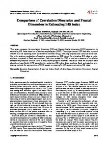
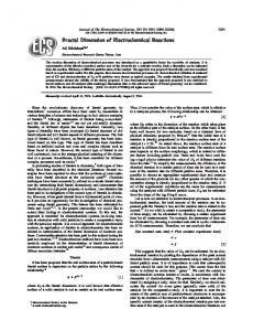
Fig. 1. Weierstrauss cosine function for FDs equal to 1.5 and 1.2.

yielding an sum of average lengths in (2)

for each

as indicated

problem by creating a general unit or yardstick: the average step or average distance between successive points, . Normalizing distances in (3) by this average results in

(2) (5) , is proportional to The total average length for scale , , where is the FD by Higuchi’s method. In the curve of versus , the slope of the least squares linear best fit is the estimate of the fractal dimension [1].

Defining as the number of steps in the curve, then and (5) can be written as

,

(6)

B. Katz’s Algorithm In contrast to Petrosian’s method (to be described in Section II-C), Katz’s FD calculation [2] is slightly slower, but it is derived directly from the waveform, eliminating the preprocessing step of creating a binary sequence. The FD of a curve can be defined as (3) where is the total length of the curve or sum of distances between successive points, and is the diameter estimated as the distance between the first point of the sequence and the point of the sequence that provides the farthest distance. Mathematically, can be expressed as

distance

(4)

Considering the distance between each point of the sequence and the first, point is the one that maximizes the distance with respect to the first point. The FD compares the actual number of units that compose a curve with the minimum number of units required to reproduce a pattern of the same spatial extent. FDs computed in this fashion depend upon the measurement units used. If the units are different, then so are the FDs. Katz’s approach solves this

Expression (6) summarizes Katz’s approach to calculate the FD of a waveform. C. Petrosian’s Algorithm Petrosian uses a quick estimate of the FD [5]. However, this estimate is really the FD of a binary sequence as originally defined by Katz [2]. Since waveforms are analog signals, a binary signal is derived following four different methods denoted with the letters , , , and , in [5], respectively. A fifth method is also included in [5], but it is the same as with an adjustable parameter. Method generates the binary sequence by assigning ones when the waveform value if greater than the mean of the data window under consideration, and zero when it is lower than the mean. In method , the binary sequence is formed by assigning one each time the waveform value is outside the band of the mean plus and minus the standard deviation, and assigning zero otherwise. Method constructs the binary sequence by subtracting consecutive samples on the waveform record. From this sequence of subtractions, the binary sequence is created by asor depending on whether the result of the subsigning traction is positive or negative respectively. In method , the differences between consecutive waveform values are given the value of one or zero depending on whether their difference exceeds or not a standard deviation magnitude. A variation of this

ESTELLER et al.: COMPARISON OF WAVEFORM FRACTAL DIMENSION ALGORITHMS

179

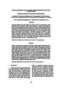
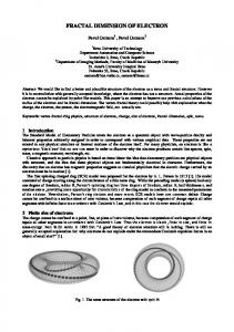
FD by each method versus theoretical FD of synthetic signal for different number of points (N ). (a) By Higuchi’s method, +++N = 150, - - - N = 250, N = 500, N = 750, -.- N = 1000, N = 2000; (b) By Katz’s method, -.-.- N = 150, N = 250, . . . N = 500, N = 750, N = 1000, +++N = 2000; (c) By Petrosian’s method “c,” N = 150, - - - N = 250, -.-.- N = 500, N = 750, +++N = 1000, . . . = 2000; and (d) By Petrosian’s method “d,” N = 150, - - - N = 250, -.-.- N = 500, N = 750, +++N = 1000, . . . N = 2000. Fig. 2. ... ---

method consists of utilizing an a priori chosen threshold magnitude different from the standard deviation, is denoted by Petrosian as method . The FD of any of the previous binary sequences is then computed as (7)

length. Each of the algorithms described above was implemented in MATLAB and tested on synthetic signals with known FD, and on experimental data derived from intracranial EEG signals of epileptic patients. Synthetic data were produced using the deterministic Weierstrauss cosine function [13], given as follows: (8)

where is the length of the sequence (number of points), and is the number of sign changes (number of dissimilar pairs) -in the binary sequence generated. III. METHODS We tested these algorithms with respect to reliability, efficiency (computational time), noise sensitivity, and record

, and we fixed and . The fractal where . A set of dimension of this signal is given by equals 100 sequences, each with different FD, was generated using (8). Fig. 1 shows two of the sequences generated. The FD of the experimental signals was computed using a sliding window approach. A total of 16 seizure records from epileptic patients was analyzed. As the sliding window moved

180


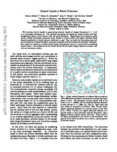
Fig. 3. Effect of noise on the FD estimate (SNR = 10 db) by (a) Higuchi’s; (b) Katz’s; (c) Petrosian’s method “c”; and Petrosian’s method “d.” (Symbols for each window length are the same used on Fig. 2.)

over the data, the FD was computed for each set of points that lay inside the window. A sliding window of 1.25 s was used to promote stationarity in each segment analyzed, considering that our EEGs were sampled at 200 Hz; the sliding window was 250 points. An overlap of 0.45 s or equivalently a displacement of 160 points was used. IV. RESULTS FDs of synthetic signals ranged from 1.001 to 1.991. Fig. 2(a)–(d) shows the FD values obtained by each of the analysis methods plotted against the known FDs of the synthetic data. Note that perfect reproduction of the known FDs should yield a straight line of slope equal to one. Higuchi’s algorithm [Fig. 2(a)] provides the most accurate estimates of the FD. Katz’s method [Fig. 2(b)] is less linear. Its calculated FDs are

exponentially related to the known FDs. Petrosian’s algorithm [Fig. 2(c) and (d)] is relatively linear and demonstrated the least dynamic range for the estimated FD (approximately between 1.01 and 1.055). Similar results are obtained for the other variations of Petrosian’s method described in Section II. The FD estimates with Higuchi’s method improve as the window length increases. No window length effect is observed in the range of 150 to 2000 points for Petrosian’s method. In Katz’s method the window length affects the dynamic range of the estimated FD yielding a dynamic range between 1 and 1.2 for window lengths greater than 750 points, and between 1 and 1.3 for window lengths lower than 250 points. The curve that is closest to the ideal straight line of slope one was obtained for a window size of 250 points. The FD results obtained with experimental EEG data reveal that even though Higuchi’s method is the most accurate of


Fig. 4.

181

FD of EEG signals for (a) Higuchi’s method, (b) Katz’s method, (c) Petrosian’s method “c,” and (d) Petrosian’s method “d.”

the three; Katz’s method yielded the most consistent results regarding discrimination between states of brain function. Specifically, when considering the distinction between the period before an epileptic seizure (preictal period) and the seizure period (ictal period), Katz’s technique provided the most repeatable and discriminative results between preictal and ictal phases over 16 EEG records analyzed [7], [8]. Fig. 3(a)–(d) presents the FD estimated for each method when the synthetic signal is contaminated with white noise, yielding a signal to noise ratio (SNR) of 10 db. Higuchi’s and Petrosian’s algorithm with binary sequence established by method “ ” [Fig. 3(a) and (c)] are severely affected by this level of noise. However, Katz’s method is influenced by the noise, but not as much as the other methods, and it turns out that its dynamic range is enhanced with the presence of noise. Another interesting observation is that when Petrosian’s algorithm is used with the binary sequence obtained by the other preprocessing methods , , , and proposed in [5], the results present even less sensitivity to the noise than Katz’s; but still maintain their reduced dynamic range. When comparing

Fig. 2(c) and (d) with Fig. 3(c) and (d), respectively, it becomes clear that the noise sensitivity in Petrosian’s method depends highly on the type of binary sequence used. Furthermore, all the binary sequences proposed by Petrosian except the one in assign the digital value of one, once a threshold or threshold band is exceeded; while the binary sequence defined in method changes from one to zero every time there is a slope sign change disregarding the magnitude of the slope sign change. Logically, when white noise is added to the synthetic signal, the variability of the signal increases and slope sign changes occur more frequently, creating a high sensitivity to the noise. Analyzes for different SNRs demonstrated that Higuchi’s and Petrosian’s algorithm when used with the slope sign change binary sequence in method , deteriorate for low SNRs; while Katz’s algorithm and Petrosian’s method when used with the threshold-based binary sequences are the most immune to the noise effects. Fig. 4(a)–(d) presents as example four records analyzed from one epileptic patient by the three FD methods introduced earlier. Equivalent results were obtained for all the records

182


TABLE I COMPARISON OF COMPUTATIONAL BURDEN AND RUN-TIME

studied. Time labeled as zero corresponds to the beginning of the ictal period. The better performance of Katz’s algorithm over Higuchi’s can be explained by two reasons. One is the exponential characteristic observed in Fig. 2(b). Because of this exponential relationship to known FDs, Katz’s method emphasizes the higher FDs, which presumably contribute the most to discriminating different states of brain function with respect to seizures. In this case, it appears that the true value of the FD is not as important as the changes in FD associated with different brain states, a feature that may be desirable in other systems or applications. The other reason can be explained from Fig. 3(a) where the high noise sensitivity of Higuchi’s method is evident. Note that the function represented in this figure has lost the one-to-one relationship between the estimated and the real FD of the synthetic signal, due to the effect of noise added. For window lengths greater than 150 points, most of the estimated FD values are the image of two different FD values. This can explain the low distinguishability of the FD over time in Fig. 4(a), conjecturing that different EEG segments with different FD values, in the presence of noise, can yield the same FD estimate when Higuchi’s method is used. In Petrosian’s method, the slope-sign-change binary sequence yielded the least distinguishability between the preictal (preseizure) and ictal (seizure) stages as is observed in Fig. 4(c). On the other hand, the threshold band-based binary sequence as defined by method “ ” yielded the most distinguishability between the preictal and ictal stages [Fig. 4(d)] among all the other threshold based binary sequences defined by Petrosian. A comparison of computational burden between the methods for different window lengths is presented on Table I. Of note is that the algorithms were reprogrammed for faster running producing an enhancement with respect to the results presented in [14]. Petrosian’s algorithm was evaluated with all its different binary sequences, but only the one described in method “ ” is presented in Table I, since it is the one that exhibit the greatest distinguishability between the pre-seizure and seizure stages. When Petrosian’s algorithm was used with the other binary sequences proposed, the running times and the floating point operations were smaller. Katz method has the highest number of floating point operations (flops), around twice the flops of Higuchi’s and one fourth more than Petrosian’s method “ ”; however, it is computationally faster for small data records. For records of 2000 points length, run-times for Katz’s and Higuchi’s are in the same order of magnitude, and Petrosian’s with method “ ” is faster. If the record length is increased further to 8000 points, then Higuchi’s algorithm becomes slightly faster than Petrosian’s and faster than Katz’s.

With respect to the fastest method (Petrosian’s for window lengths between 500 and 4000 points), Katz’s lags by 35.2% and Higuchi’s by 66.4%, when using a window length of 500 points. This is not a problem since the total record length analyzed is 12 min long; therefore, all three methods can be run in real time. If the window length increases up to 8000 points, then Higuchi’s performance improves and becomes 3.7% faster than Petrosian’s. V. CONCLUSION Our results show that Katz’s algorithm is the most consistent method for discrimination of epileptic states from the IEEG, likely due to its exponential transformation of FD values and relative insensitivity to noise. Higuchi’s method, however, yields a more accurate estimation of signal FD, when tested on synthetic data, but is more sensitive to noise. Petrosian’s method performance depends on the type of binary sequence used. If a binary sequence based on slope-sign-changes is utilized then this method becomes less suitable for analog signal analysis, given its high sensitivity to noise and its poor reproducibility of dynamic range of synthetic FDs. This study demonstrates that a careful selection of FD algorithm is required for specific applications. Factors such as knowledge of possible FD range, noise level, and window length must be considered to achieve the best results. ACKNOWLEDGMENT The authors would like to thank C. Bowen and R. Shor for their help in the data generation. They also want to acknowledge and thank the reviewer for several fruitful suggestions. REFERENCES [1] T. Higuchi, “Approach to an irregular time series on the basis of the fractal theory,” Physica D, vol. 31, pp. 277–283, 1988. [2] M. Katz, “Fractals and the analysis of waveforms,” Comput. Biol. Med., vol. 18, no. 3, pp. 145–156, 1988. [3] A. Accardo, M. Affinito, M. Carrozzi, and F. Bouquet, “Use of the fractal dimension for the analysis of electroencephalographic time series,” Biol. Cybern., vol. 77, pp. 339–350, 1997. [4] V. Cabukovski, N. d. M. Rudof, and N. Mahmood, “Measuring the fractal dimension of EEG signals: Selection and adaptation of method for real-time analysis,” in Second Int. Conf. Computers in Biomedicine, Computational Biomedicine, 1993, pp. 285–292. [5] A. Petrosian, “Kolmogorov complexity of finite sequences and recognition of different preictal EEG patterns,” in Proc. IEEE Symp. Computer-Based Medical Syst., 1995, pp. 212–217. [6] N. Pradhan and D. N. Dutt, “Use of running fractal dimension for the analysis of changing patterns in electroencephalograms,” Comput. Biol. Med., vol. 23, no. 5, pp. 381–388, 1993.


[7] R. Esteller et al., “Fractal dimension characterizes seizure onset in epileptic patients,” in Proc. 1999 IEEE Int. Conf. Acoustics, Speech, Signal Processing, Phoenix, AZ, 1999. , “Fractal dimension detects seizure onset in mesial temporal lobe [8] epilepsy,” in Proc. 21st Annual Int. Conf. IEEE Eng. Medicine Biol. Soc., Atlanta, GA, 1999. [9] N. H. Packard, J. P. Crutchfield, J. D. Farmer, and R. S. Shaw, “Geometry from a time series,” Phys. Rev. Lett., vol. 45, pp. 712–716, 1980. [10] F. Takens, “Detecting strange attractors in fluid turbulence,” in Dynamical Systems and Turbulence, D. a. y. L.-S. Rand, Ed. Berlin, Germany: Springer-Verlag, 1981, vol. 898, (Lecture Notes in Mathematics), pp. 366–381. [11] P. Grassberger and I. Procaccia, “Characterization of strange attractors,” Phys. Rev. Lett., vol. 50, no. 5, pp. 346–349, 1983. [12] C. Elger and K. Lehnertz, “Seizure prediction by non-linear tiem series analysis of brain electrical activity,” European J. Neuroscience, vol. 10, pp. 786–789, 1997. [13] C. Tricot, Curves and Fractal Dimension. New York: Springer-Verlag, 1995. [14] R. Esteller, G. Vachtsevanos, J. Echauz, and B. Litt, “A comparison of fractal dimension algorithms using synthetic and experimental data,” in Proc. 1999 IEEE Conf. Circuits Systems, Orlando, FL.

Rosana Esteller (S’98) received the B.S.E.E. and a M.S.E.E. degrees from the Simón Bolívar University, Caracas, Venezuela, in 1986 and 1994, respectively, and the Ph.D. degree in electrical engineering from Georgia Institute of Technology in 2000. Currently, she is Assistant Professor at the Simón Bolívar University. Her research interests are in applications of signal processing techniques from linear and nonlinear dynamics for detection, prediction, classification, pattern recognition, modeling, and estimation of signals and systems. Particular interest in applications to biomedical signals and intracranial EEG signals from epileptic patients. She is a member of Sigma Xi.

George Vachtsevanos (S’62–M’63–SM’89) received the B.E.E. degree from the City College of New York, the M.E.E. degree from New York University, and the Ph.D. degree in electrical engineering from the City University of New York. He is currently a Professor in the School of Electrical and Computer Engineering at the Georgia Institute of Technology where he directs the Intelligent Control Systems Laboratory. His research interests include intelligent systems, diagnostics and prognostics, robotics, and manufacturing systems. Dr. Vachtsevanos has published in the areas of control systems, power systems, bioengineering, and diagnostics/prognostics. He is a member of Eta Kappa Nu, Tau Beta Pi, and Sigma Xi.

183

Javier Echauz (S’93–M’95) was born in San Juan, Puerto Rico. He received the B.S.E.E. degree in 1988 from the University of Puerto Rico–Mayagüez (UPRM), and the M.S.E.E. and Ph.D. degrees in 1989 and 1995 from Georgia Institute of Technology. At Georgia Tech, he held the Georgia Tech President’s Fellowship, the GEM, Du Pont, and GTE fellowships, and a scholarship from the Economic Development Administration of Puerto Rico. During 1998 and 1999, he was an Associate Director of the Electrical and Computer Engineering Department at UPRM, and is currently an Associate Professor under leave of absence from that institution. He has been involved in quantitative EEG analysis and research for the past 9 years. His current research interests center around intelligent devices for epilepsy.

Brian Litt (A’88–S’89–M’91) received the A.B. degree in engineering and applied science from Harvard University in 1982 and the M.D. degree from Johns Hopkins University in 1986. Residency in Neurology, Johns Hopkins University, 1988–1991. Neurology Faculty, Johns Hopkins Hospital, 1991–1996. Neurology/Biomedical Engineering Faculty, Emory University/Georgia Institute of Technology 1997–1999. Dr. Litt is an Assistant Professor of Neurology; Assistant Professor of Bioengineering, Director, EEG Laboratory and Epilepsy Surgery Program University of Pennsylvania. His scientific research is focused on his clinical work as a Neurologist specializing in the care and treatment of individuals with epilepsy. It encompasses a number of related projects: 1) automated implantable devices for the treatment of epilepsy, 2) seizure Prediction: developing an engineering model of how seizures are generated and spread in human epilepsy, 3) localization of seizures in extratemporal epilepsy, and 4) minimally invasive tools for acquisition and display of high fidelity electrophysiologic recording.