92
Int. J. Creative Computing, Vol. 1, No. 1, 2013
A creative computing approach to 3D robotic simulator for water pollution monitoring John Oyekan Centre for Research into Distributed Technologies, University of Bedfordshire, Luton, LU1 1JN, UK E-mail:
[email protected]
Bowen Lu and Huosheng Hu* School of Computer Science and Electronic Engineering, University of Essex, Wivenhoe Park, Colchester CO4 3SQ, UK E-mail:
[email protected] E-mail:
[email protected] *Corresponding author Abstract: This paper presents a creative computing approach to the development of a 3D robotic simulator that could be used to develop control algorithms for a team of robotic fishes to effectively monitor water pollution. The computational fluid dynamics of a marine environment is taken into consideration, which differs from most existing robotic simulators and shows its creativity. It is the first 3D robotic simulator that enables users to develop control and navigation algorithms for pollution monitoring by a school of biologically inspired robot fishes. Additionally, this simulator has an interface to force fields and provides the diversity of simulation scenarios. The recordand-replay strategy is deployed in the simulator so that the fluid computation is done offline and recorded into a log file, which can then be replayed during a simulation. Experiments were conducted and results show that the proposed approach is feasible and has potential to be developed for a wider range of underwater applications. Keywords: creative computing; 3D simulator; robotic fish; autonomous navigation; pollution monitoring; Panda3D. Reference to this paper should be made as follows: Oyekan, J., Lu, B. and Hu, H. (2013) ‘A creative computing approach to 3D robotic simulator for water pollution monitoring’, Int. J. Creative Computing, Vol. 1, No. 1, pp.92–119. Biographical notes: John Oyekan received his PhD in Robotics from the University of Essex, UK. He is currently a Senior Research Fellow with the Centre for Research in Distributed Technologies, University of Bedfordshire, Luton, UK. He has published over 12 international conference and journal papers including co-authoring two book chapters. His current research interests include robotics, computational intelligence, multi-agent systems, unmanned aerial vehicle control, and computational neuroscience. He has served as a reviewer for IEEE ROBIO, IROS, ICRA, among others. He is also a member of the programme committee for IEEE ROBIO 2012.
Copyright © 2013 Inderscience Enterprises Ltd.
A creative computing approach to 3D robotic simulator
93
Bowen Lu is a PhD candidate in the School of Computer Science and Electronic Engineering, University of Essex, UK. He received his BEng in Optical Information Science and Technology from Shenzhen University, China in 2008 and his MSc in Embedded Systems from University of Essex in 2009. Currently, he is researching on various distributed methods for pollution monitoring, including coverage control algorithms for wireless sensor networks and pollutant distribution estimation. He has served as a reviewer of IEEE ICRA, IROS and other international conferences. He is a student member of IEEE. Huosheng Hu is a Professor in the School of Computer Science and Electronic Engineering, University of Essex, UK, leading the human-centred robotics research. His research interests include autonomous robots, human-robot interaction, rehabilitation robotics, embedded systems, multi-robot collaboration, pervasive computing, sensor integration, intelligent control and networked robotics. He has published over 380 papers in journals, books and conferences, and received a number of best paper awards. He is a founding member of IEEE Robotics and Automation Society Technical Committee on Networked Robots, a fellow of IET and InstMC and a senior member of IEEE and ACM. He currently serves as an Editor-in-Chief for International Journal of Automation and Computing, Founding Editor-in-Chief for Robotics Journal, and Executive Editor for International Journal of Mechatronics and Automation.
1
Introduction
Recently, many researchers are investigating how robotic agents could be used to monitor the water quality in lakes, rivers and seas around the world. In particular, some bioinspired robotic fishes equipped with advanced navigation algorithms have been developed based on biological inspiration. These bio-inspired robotic fish are able to monitor water pollution cooperatively so that their chances of finding a pollution source can be greatly enhanced. Figure 1 shows a robotic fish platform developed at the University of Essex, which can swim as a real fish peacefully and navigate in water autonomously. In order to develop control and navigation algorithms for these robotic fish, a 3D simulator is needed so that the developed algorithms can be tested before their deployment on physical platforms for pollution monitoring. There are many different 3D simulators have been developed for multi-robot systems over the years, which are in the forms of custom-based and commercially available simulators. For example, Tu (2000) developed a custom simulator in order to investigate fish behaviours. Liu and Hu (2004, 2010) developed a simulator to generate and test different swim motion patterns so that they can be used on a physical robotic fish effectively. Nawaz et al. (2010) developed a simulator to test a sensor monitoring system that was to be deployed to monitor underwater nuclear storage pools. However, these simulators assume that robotic fish work in a static environment and no disturbance or turbulence affects the plume or pollutant concentration generated by a pollutant source.
94
J. Oyekan et al.
Figure 1
The robotic fish platform (see online version for colours)
Source: Hu et al. (2006)
In order to introduce disturbance into the environment, a laminar flow field or a random number generator could be deployed without the consideration of the environment structure. If the environment structure must be taken into consideration, computational fluid dynamics (CFDs) should be used in the simulator. However, CFDs simulations are computationally expensive and difficult to be implemented in real time. Farrell et al. (2002) were able to solve this problem partially by using a set of CFDs equations with a colored noise process but no environment structure was taken into consideration. This led to a plume that meandered in the flow field but did not interact with the physical environment. This method was deployed in Zarzhitsky et al. (2005), where the code was developed in an environment with obstacles and resulted in plume interaction and meandering. In addition to studying the effect of the developed swarm algorithms, the simulator should also enable the study of the effect of the hydrodynamics of the robotic fish platform on the plume structure, as well as effect of acoustic communication issues on the algorithm among other factors. Results from these studies could then be used to improve the performance of the robotic fish platform and the swarm algorithm. As the robotic fish would be operating in a 3D underwater environment, a 3D simulator should be deployed to carry out the studies mentioned above. The existing simulators on the market have no functionality needed for generating the pollutant particles and the plume structure of pollution effectively. For instance, the Webot simulator is a 3D commercial simulator that has been around for over ten years (Cyberbotics, http://www.cyberbotics.com/overview). It includes robot models for Pioneer robots (Adept Mobile Robots, http://www.mobilerobots.com/researchrobots/researchrobots/pioneerp3dx%.aspx), Sony AIBO robots (Sony, http://www.sonyaibo.net/aboutaibo.htm), Kephera robots (K-Team, 2011), but can not be used for underwater robots. MobileSim is another existing simulator provided by ARIA, which has no models for the robotic fish. Simbad (http://simbad.sourceforge.net/) is a 3D simulator developed in Java, which cannot achieve real-time performance.
A creative computing approach to 3D robotic simulator
95
Hence it is necessary to creat a custom 3D simulator with a full control over the development process, including the introduction of various CFDs, flow fields, sensor models, custom built robots and so on. Panda3D (Mellon, 2011) is selected as a suitable platform to develop such a creative simulator, which has the following features: •
It is an open source game engine developed in Python scripting language. This language has a lot of support in the research community making it possible to use readily available codes to aid the simulator development and reduce development time.
•
Python could be written in object-oriented programming (OOP) style which makes it easy to maintain and suitable for developing software with complex framework.
•
Panda3D has C++ cross-language interface, which provides more completed ability on general programming and kernel algorithm developing.
•
It comes with a physics engine that enables collision between objects to be detected and addressed accordingly.
•
Recently, a bunch of artificial intelligence modules that comprises of behaviours such as flocking, obstacle avoidance, pursuing, etc., has been added. These advanced behaviours could be helpful on simplifying the lower level coding works.
•
The use of textures on objects in Panda3D is very easy and so is camera control. It also offers integration with model development software such as Blender, 3DMax and so on. In other words, the use of Panda3D encouraged flexibility that was needed in this project to achieve various goals.
The rest of this paper is organised as follows: in Section 2, the project requirements and specifications are discussed. Section 3 discusses how various tools were used with Panda3D to construct a creative 3D simulator. In Section 4, the proposed approach is tested and various control algorithms are evaluated in the simulator. Finally, a brief conclusion and future work to be carried out are given in Section 5.
2 Project requirements and design thinking This section aims to present the requirements that the simulator to be constructed should meet. In order to do this, the functional requirement in the form of a set of shall statements in Section 2.1 was first constructed. Following this, the functional parts of the simulator are discussed with how they would link together in a software architectural diagram as presented in Section 2.2. The software design and design phases are illustrated in Section 2.3.
2.1 Functional requirements: shall statements In this section, the proposed final status for the simulator is presented. The simulator:
96
J. Oyekan et al.
•
shall be able to simulate a representation of the robotic fish in a marine environment
•
shall provide an interface so that various developers can add and develop their control codes
•
shall simulate the fluid dynamics of an underwater environment
•
shall be able to switch between different flow regimes representing different peclet numbers
•
shall simulate the pollution conditions at various peclet numbers
•
shall simulate pollution leaking from an underwater pipe and ships
•
shall simulate different categories of pollutant released into the water
•
shall simulate pollution dispersion as a result of waves, currents, and passing ships
•
shall be able to change the flow parameter values of the simulated river
•
shall take interaction between different objects into consideration
•
shall take the physical properties (e.g., viscosity, density, etc.) of the pollution transportation medium into consideration
•
shall ensure that computation time is efficient enough to enable real time interaction with objects in the simulator
•
shall make sure that there is an interface to which a user can comfortably interact with.
2.2 Software architecture Figure 2 presents the software architecture that was designed during the writing of the requirements and specifications for the simulator. This architecture shows the components needed to achieve the task, including the communication and relationship among components. •
Force field (or fluid velocity) database manager is designed as a bunch of CFD simulated records from OpenFOAM, which gives the flowing information of the water body in the port, and its content is a grid map of force vectors. CFD is a time consuming job, this design moves the computation to a separate offline block to guarantee the real-time feature of the designed simulator.
•
A physics engine is a library that provides an approximate simulation of certain simple physical systems, such as rigid body dynamics (including collision detection), soft body dynamics, and fluid dynamics, of use in the domains of computer graphics, video games and film. The physics engine module processes interactions of forces on each object. It reads the force field information from the database, applies constant forces (including force of gravity and buoyancy, etc.), and eventually outputs position change information for all objects. The physics engine is connected to the pollution module and the moveable objects module
A creative computing approach to 3D robotic simulator
97
(robotic fish and ships). This module is not compulsory if the robotic fishes or other moving objects implemented their own simplified algorithms instead of using physics engine. This is usually encouraged that some functions in physics engine contain huge amount of computation, e.g., collision detection. •
Pollution model module is a collection of pollution models, which has different diffusion behaviours, according to the properties of leaking pollutants. These models will be synthesised with force field information through the physics engine interface and update the pollutant distribution.
•
Ship dynamics algorithm module simply moves ship objects (potential leaking source) around the port according to a prefixed or random path.
•
Robotic fish control algorithm module is a set of pollution monitoring algorithms for mobile sensor networks, which is the kernel of detecting pollution distribution. Currently, BCT-FLK and DSVR-CVT would be investigated as potential algorithms to be used and tested on the robotic fish platform (Lu et al., 2010; Oyekan et al., 2010). This module reads the positions of robotic fishes and pollutant concentration of current position as input to optimise the distribution of robotic fish. As a design feature, the control algorithms can be written in any language supported by Python, however, need to provide the unified information required by the simulator.
Most of the computations are contained in the physics engine and pollution models. Depending on the computational demands, these two parts should be substituted with the simplified algorithm or developed in some efficient language, e.g., C++ (compiling languages). They could also be compiled into a dynamic link library files with standard interface so that they can be used in different simulator environments. This module-based design provides better team development feasibility, and would be easier to maintain in the future.
2.2.1 Real-time 3D animation The current graphic process units (GPU) is still not fast enough for a synchronous real-time simulation with a large scale complex 3D environment. Hence a front-back asynchronous design should be introduced to this simulator, where a 3D environment animation would be running in the front end while the CFDs field and pollution monitoring algorithms would be running in the back end. The back end is the kernel of simulator, which can actually run individually (without front end). In this design structure, the 3D animation is isolated from the pollution monitoring algorithms’ feedback loop resulting in a clarification of each function into modules. Without the interference from the 3D animation, collision detection in the physics engine can be replaced with user defined collision avoidance algorithm. This is because the physics engine collision detection could result in heavy computational burden as a result of keeping track of various objects in the simulator. The three major designed features are detailed below: •
Front-back ends design. Back-end runs pollution monitoring algorithm (pollution distribution estimation), and front-end visualises the simulation results in 3D animation together with other contour plots.
98
J. Oyekan et al.
•
Front and back ends are running in different frequency rate (asynchronous design). The update frequency of back-end algorithms are designed to synchronous with time, and the front-end update frequency is normally lower (with a lower FPS, the real-time feature of the simulator is achieved).
•
Collision detection could be disabled, using the collision avoidance behaviour from control algorithm only.
Figure 2
The proposed software architecture (see online version for colours)
2.3 Software design and build phases 2.3.1 Interfaces The interfaces shall be capable of loading various port models, fluid velocity fields, pollution models, and pollution monitoring/control algorithms in different programming
A creative computing approach to 3D robotic simulator
99
languages. In order to make sure that this simulator is extendable for further development, the Python language was chosen as the choice of design language. Python has a fast development speed building on an OOP framework, and supports various other main trend languages. One port model, one pollution model, and two pollution monitoring algorithms would be tested and used first. They could also be extended to all Python supported languages. Currently a BCT-FLK algorithm coded in Python and DSVR-CVT coded in C++ are used to test integration with other languages. On the other hand, a 3D physics engine and animation package, Panda3D, are supported by Python.
2.3.2 Potential capability Blender is chosen for building all 3D models and animations for port and robotic fishes. For current stage, the main purpose of current development is testing and demonstrating the efficiency of high level control algorithms, a point model is employed and the 3D animation of swimming fish is applied on top of each point model. In order to have a low level kinematic model implemented, the shape and joint information is needed, and then, Blender can be used to build the shape and joint parameters precisely. It shows that Blender is capable for building the joint-based models.
2.3.3 Design phase By following the discussions above, a working plan can be produced in sequence as follows: •
create 3D animation models for fish and water environment. Later we will consider additional models for port, ship, and, etc. (Blender)
•
develop customised simple physics engine dynamic link library. (C++)
•
build 3D simulator modules in Python. (Blender together with Panda3D)
2.4 Summary In this section, the software requirement for the simulator has been briefly presented, together with the software architecture to build the simulator. In addition, the issues that could arise during the development and testing of the simulator have been presented with possible solutions to these issues. In the next section, the process of building the simulator would be presented.
3 Simulator development After describing the requirements needed by the simulator above, the tools for developing the simulator were chosen for the simulator development, and a location was chosen as a test site to compare obtained results. The location chosen was near the University of Essex, i.e., University Quays Accommodation where the River Colne flows past as shown in Figure 3.
J. Oyekan et al.
100 Figure 3
The River Colne at the University Quays in Colchester (see online version for colours)
This location was chosen because of its accessibility thereby making it possible to compare the natural flow field with a flow field simulated from OpenFOAM. Also, this location is affected by the tidal effect from the Black sea making it possible to view its bed when the tide is low. This made it possible to develop a representation of the 3D map of the river bed in addition to its boundaries. Furthermore, the area chosen is affected by various flow regimes including turbulent flow regimes. As a result, different sections of the area would have different flow regimes making it possible to test the behaviour and performance of developed algorithms in various scenarios.
3.1 Architecture and framework As mentioned in the introduction section, Panda3D was considered as a suitable tool to develop the robotic fish simulator. As a supplement to Panda3D, a series of other tools were also considered and used. The framework shown in Figure 4 was used to combine the tools, in which (a) shows the framework of the simulator from the view of data flow and (b) shows the steps of constructing a port model. •
In order to develop the simulator, a picture of the environment, as shown in Figure 3, was first taken. This picture was then used in Blender and OpenFOAM CFDs package.
•
Blender is an open source development package that can be used to develop 3D worlds and introduce various effects (Blender, http://www.blender.org/). Blender also incorporates a physics game engine and particle system which makes it possible to introduce interactions between various objects in the simulated environment and also create smoke, moving water and other similar effects. However, it was discovered that there was no control over each individual particle in a user developed particle system. As a result, it was impossible to control the shape of a simulated pollutant plume.
A creative computing approach to 3D robotic simulator
101
Figure 5 was the created 3D model by Blender, according to the environment of interest by using the picture taken as shown in Figure 3. The environment developed was set up in Blender so that when imported into Panda3D, the boundaries of the environment could act as actual physical boundaries to prevent objects from going through them. This was achieved by using the ‘chicken exporter’ tool in Blender. In developing the robotic fish, a bone frame based on a 3D fish model was used as shown in Figure 6. In this design, each of the joint is customisable, including the quantity and organisation of the bones. Although we are using a point model for fish movements at the current stage, this bone frame can potentially support kinematic methods in the future work. •
OpenFOAM (Jasak, 2009) is an open source CFDs programme that incorporates its own mesh generators, e.g., snappyHex and blockMesh. The process of meshing simply converts an environment into grids or cells that enable the computer to perform finite element method (FEM) computations across the environment of interest. The environment shown in Figure 3 was simplified and converted into a mesh as shown in Figure 9(a). In order to perform CFDs, equations that govern the flow of fluid in the environment have to be derived. The choice of these equations would depend on whether the fluid is to be turbulent, laminar, viscous, incompressible and so on. After the equation to describe the fluid has been chosen, the environment is divided up discretely using a mesh generator so that the fluid equation could be solved discretely for the various areas in the environment (Jasak, 2009). Figure 7 shows textured fish model. As mentioned above, we created a series of animation of swimming fish in different flipping frequency for different moving speeds. Depending on the size of the environment and the resolution of the meshes, the results from the computational fluid simulation could take up to days. As a result, it is very challenging to perform real time CFDs of an environment without incurring computational overheads. In order to obtain CFDs results more quickly, the environment to be simulated was reduced by a factor of 10 before expanding back into normal real life dimensions. The results of doing a CFDs computation on Figure 9(a) is shown in Figure 9(b). The structure of OpenFOAM enables users to easily establish different flow regimes ranging from laminar to turbulent by setting flow parameters in equations. For more information, the reader is referred to the OpenFOAM manual at Jasak (2009). OpenFOAM was used to generate flow field data which was then used in Panda3D to advect pollution particles and affect the dynamics of the Robots in the simulator.
•
With the framework shown in Figure 4, it was possible to make a module that could incorporate various controllers for testing on physical robots in Panda3D.
102 Figure 4
J. Oyekan et al. Developing the Robotic fish simulator, (a) simulator data flow (b) port construction flow
(a)
(b)
Figure 5
The simulated River Colne at the University Quays (see online version for colours)
A creative computing approach to 3D robotic simulator Figure 6
Bone frame of fish model (see online version for colours)
Figure 7
Textured fish model (see online version for colours)
103
3.2 Development of plumes In a running river, a pipe leaking a pollutant would result in the formation of a plume. In order to reproduce a plume in these studies, an environment was constructed as shown in Figure 9. The environment had dimensions of 400 by 1, 000 with obstacles being placed in it to generate its boundaries. CFDs simulation was then performed on this environment using OpenFOAM CFDs package. Flow vectors were obtained from the simulation carried out. The use of particles for simulating smoke can be found in many simulations and animations. Many existing theories use particles such as Smoothed-particle hydrodynamics (SPH). However, the downside of using particles to simulate smoke is that many particles are required to simulate realistic smoke, which results in a heavy computational burden. Another way of simulating pollution is through the use of various models such as puff models or Gaussian models. The disadvantage of using the Gaussian model is that it is difficult to control the resolution of the movement of a section of plume. However, by combining these two theories together, it is possible to achieve a system in which the particles can be controlled as in a normal smoke simulation and also achieve a plume like effect by using it with Gaussian-based model. As a result, the plume puffs in this work were constructed from a Gaussian distribution of particles around a mean point µ that was advected from the plume source according to the flow field. The spread or standard deviation ω of the distribution of particles was increased according to equation (1) where k is a constant that can be tuned to the user’s preference. ωt+1 = ωt + kt
(1)
Figure 8
J. Oyekan et al. (a) The meshed simulated environment (b) The velocity vectors obtained from OpenFOAM advecting a particle in the simulated marine environment (see online version for colours)
(a)
120
100
80
Y
104
60
40
20
0
0
5
10
15
20
25 X
(b)
30
35
40
45
A creative computing approach to 3D robotic simulator Figure 9
Figure 10
105
Test environment
Simulated robotic fish deployed in the 3D simulator (see online version for colours)
In this way, the plume shown in Figure 9 was obtained. By multiplying the flow vectors with either a constant or random value, it is possible to control the x and y speeds of the plume resulting in either a defined plume with a predictable path or a meandering plume. In this case, the x and y speeds, xv and yv , were set to 14 times their scalar values. In Figure 9, it can be observed that the plume was more patchy towards the source. This is because the flow field energy was strong in the narrow space. However this energy dissipated after the area enlarged resulting in a less patchy section of the plume. This energy was slightly regained in the lower section of the simulated environment resulting in a patchy plume again. The plume development approach was then tested in a 3D underwater environment with the robotic fish deployed in it as shown in Figure 10.
106
J. Oyekan et al.
3.3 Summary This section has briefly discussed the processes involved in the development of the simulator for the robotic fish. It discusses how various tools were combined and the results obtained. The results show that it has potential for use in the real-world applications.
4 Algorithm development in the simulator In this section, two different bio-inspired controllers were compared to test the approach discussed in Section 3 to the development of a robotic fish simulator. They were a diffusion-based controller based upon the bacteria behaviour and a flow-based controller based upon a male moth behaviour. The experiments were firstly conducted in a 2D environment before testing in a 3D environment.
4.1 Experiments in a 2D environment 4.1.1 Diffusion-based controller There have been various investigations into the development of controllers that can operate in diffusion like environments. For example, Mayhew (2008) used inspiration from a line minimisation-based algorithm to develop a robust source-seeking hybrid controller. In their work, gradient information and exact coordinates of the vehicles (for vehicles in GPS denied environments) were not needed. Baronov and Baillieul (2008) developed a hybrid reactive control law that enables an agent to ascend or descend along a potential field. Moreover, some researchers have looked towards nature and taken inspiration from the bacteria as in Marques et al. (2002) and Dhariwal et al. (2004). Marques et al. (2002) compared a rule-based bacteria controller with the silkworm algorithm amongst other algorithms while in Dhariwal et al. (2004), Dhariwal et al. used a keller segel model of bacteria population as an inspiration to develop a source seeking controller. In this section, Brown and Berg (1974) model was deployed because of its ease of analysis and ability to compare the behaviour of the bacteria algorithm driven robots with biological results. In addition, this model was chosen over other models such as the one in Yi et al. (2000) because it was deemed sufficient to implement a biased random walk. Furthermore, it gives the user the ability to control both the exploratory and exploitation behaviours of robotic agents through the tuning of its parameters. The bacterium motion is governed by a series of tumbles and run phases. A run phase can be viewed as a straight line for simplicity purposes while the tumble phase can be viewed as re-orienting itself to a randomly chosen direction. When the bacteria is moving towards a favorable food source, the run phase is increased in duration whilst if moving in an unfavourable direction, the tumble phase is increased. This was discovered and modelled by Berg and Brown according to equations (2) to (4). ) ( dPb τ = τo exp α dt
(2)
A creative computing approach to 3D robotic simulator dPb −1 = τm dt
∫
t −∞
dPb exp dt′
(
(t′ − t) τm
kd dC dPb = dt (kd + C)2 dt
107
) dt′ ,
(3)
(4)
τ is the mean run time and τo is the mean run time in the absence of concentration gradients, α is a constant of the system based on the chemotaxis sensitivity factor of the bacteria, Pb is the fraction of the receptor bound at concentration C. In this work, C was the present reading taken by the robotic agent. kd is the b dissociation constant of the the bacterial chemoreceptor. dP dt is the rate of change of Pb . dPb dt
is the weighted change rate of Pb , while τm is the time constant of the bacterial system. The above equations determine the time between tumbles and hence the length of the run phase between tumbles. During the tumble phase, the agent can randomly choose a range of angles in the uniform distribution σε{0..., 360}. In addition to the above equations, we also use a ‘foraging equation’ that controls the velocity of agents. This equation enables agents to dwell longer in areas of high pollution concentration and shorter in areas of low pollution concentration. It is presented in equation (5) where β is the dynamic velocity that depends on the present reading of the pollution C, βo is the standard velocity without any reading and vk is a constant for tuning the dynamic velocity β. β=
βo ∗ vk C
(5)
The bacteria controller does not rely on flow information and needs only a pollution measuring sensor.
4.1.2 A flow information controller Most controllers that use flow information in navigating towards the source of a pollution are inspired by the moth behaviour. Examples include the spiral surge algorithm developed by Hayes et al. (2002) and casting algorithms developed by Li et al. (2001). The spiral surge algorithm is suitable for high turbulent conditions in which there are patchy distributions of pollution. Nevertheless, the flow information controller that was chosen in this investigation was the one developed in Li et al. (2001) because of its performance in field trial tests. The passive strategy for maintaining contact with plume was chosen. The strategy relies on having a sensor that reads both. Whenever the pollution sensor detects a value above threshold υ, the agent gets the flow information in its immediate vicinity and moves upstream. As mentioned previously, chemicals in a turbulent environment often undergo ‘tearing’ leading to a patchy distribution in addition to meandering in a non-uniform environment. As a result of the patchiness of the plume, it is possible that the agent might not have any reading during its upstream travel for sometime even though it is on course towards the source of the plume. In order to solve this, a constant κ is used. If the pollution sensor reading C at time t has been above the threshold υ for the last κ seconds tϵ[t − κ, t], then it is assumed that the agent is still in contact with the plume and upstream motion is continued. Every
108
J. Oyekan et al.
time an above threshold reading is obtained, a variable TLAST is set to the current time t. Another variable called TLOST is used to determine when the plume is lost and is calculated by using TLOST = TLAST + κ. When TLOST is equal to TLAST + κ, the agent tries to reacquire the plume by going at 90◦ to the present direction of the agent. This is carried out by using equations (6) and (7) where ζv is the commanded heading of the vehicle, ζu is given by equation (8) and ψ can be either −90 or +90 depending on equation (7). The agents use equation (8) to go upstream and this is obtained by adding 180◦ to the instantaneous wind direction ζw . ζv (t) = ζu (t) + sign(ψ) { +90 ψ= −90
if if
ζv (Tlost ) − ζw (Tlost ) > −180◦ ζv (Tlost ) − ζw (Tlost ) < −180◦
ζu (t) = ζw (t) + 180
(6)
(7)
(8)
In this investigation, κ was set to 1,000 ms and υ set to 1. More information on the flow controller and its pseudo code implementation can be found in Li et al. (2001).
4.1.3 Particle filter localisation based on CFD Underwater localisation is often a very challenge task in realistic scenarios since it cannot use GPS signals. Therefore, underwater localisation relies on acoustic signals from floating buoys present on the surface of water. Using the known buoys in the environment, it is possible to localise the robotic fish in an underwater environment. In this paper, we investigated the possibility of making use of an history of flow information from a database or CFDs information about an area for localisation of the robotic fish. It might be argued that the use of CFDs is far from being realistic, however, in McEvoy and Southall (2000), the authors were able to show that results from CFDs provided close enough observations to an air supply ventilation window. The proposed use of CFD for robotic fish localisation is an inspiration taken from the Mexican cave blind fish in that it uses flows in the environment to detect obstacles in the environment and to visualise its environment (Windsor et al., 2010). In doing this, we assume that the robotic fish is equipped with accelerometers having noise and drift components as shown in equation (9) where Ω is the accelerometer reading and σ(x) is the noise and drift component. Ω := Ω + σ(x)
(9)
The location estimation algorithm is based upon the particle filter theory. Particle filter has been used in a number of applications in the past decade (Rekleitis, 2004). In this work, we modify the theory for localisation using a history k of trajectory data. The value of k was set to 4. We did not use point information because this did not give good enough estimation. A number of particles N were deployed randomly in the simulated arena. Every time step, each individual particle was advected based upon the flow field at its position. The error between the noisy velocity reading obtained by the accelerometer according
A creative computing approach to 3D robotic simulator
109
to equation (9) and the velocity of the particle was calculated. The error was added to a running error integration of that particle. A Gaussian Kernel was then used to compute the weight that each particle would contribute to the estimated position and then using arranged in order of priority with the lowest error particle having a higher weight. Using a threshold value T , any particles below the threshold are replaced by another particle placed randomly in the environment. The surviving particles are used to compute a weighted average of the estimated position of the robot. Figure 11 Arrangement of PSO and CFD database for robotic fish position estimation
4.2 2D simulation results 4.2.1 Flow controller results The oval agents representing those using the flow controller method were placed in a well established plume as shown in Figure 13(a) with the blue square indicating the source. It was discovered that all the agents were able to find the plume source for this method with an average iteration of 230. However, for the bacteria controller, the technique failed to follow the plume as shown in Figure 14(a). The boundaries of the environment were deliberately not considered in this experiment for the comparison purposes. Reliance on the gradient information makes the bacteria controller fail because it is not possible to get that information in such a turbulent environment. Nevertheless, it was discovered that if the straight runs were modified into circular casting motions by using a biological inspired step angle of σ ϵ 59 degrees ± rand() based on tracking a falling algae, it is possible to obtain an emergent characteristic, as shown from Figures 14(b) to 14(d). This characteristic enabled some agents to find the source even though a larger number of iterations (over 5,000) are required. Compared to the flow controller method, it still forms the shape of the plume as shown in Figure 14(d), in which the plume was deliberately left out to show that the agents followed the structure of the plume. This behaviour was obtained by using the bacteria parameters kd = 1, 000, α = 500, τo = 2, βo = 6 in order to achieve more exploitation in the plume than the exploration of the environment. Another emergent property discovered was that the agent stopped moving when an agent got to the source. Stopping at the source was something not programmed into the agent’s behaviour. This property could be as a result of the kd parameter being saturated and could be used as a way of declaring the source of the plume.
110
J. Oyekan et al.
Figure 12 Showing stages of the agents finding the source of the plume using the flow controller method (see online version for colours)
(a)
(b)
(c)
(d)
(e)
(f)
A creative computing approach to 3D robotic simulator Figure 13 (a) Agent distributions for ordinary bacteria behaviour (b–d) modified bacteria behaviour and for (e–f) modified bacteria behaviour with negative gradient (see online version for colours)
(a)
(b)
(c)
(d)
(e)
(f)
Notes: Red was used for the square shaped agents so that it could stand out of the black boundary. Their size was also made smaller so that the forming of the shape of the plume could be seen more clearly.
111
112
J. Oyekan et al.
By changing the sign in equation (4) to negative as in − dC dt , it was possible to make the bacteria dwell on the outskirts of the plume as shown in Figures 13(e) and 13(f). In this case, the agents were always pushed to the boundary of the plume whenever they came into contact with the plume. This behaviour could be used to contain the pollution plume whilst tracing its shape and moving to the source.
4.2.2 CFD particle swarm results Initial experiments were conducted using a threshold T = 14, N = 150. Assume that the fish was flowing freely down stream in estimating the position of the fish. Figure 14 shows the results obtained. Error in the estimation of the x and y axes reduces with time using the proposed approach. Figure 14 PSO versus robot fish trajectory (see online version for colours) 900
Robot path PSO Estimation
800
700
Y axis
600
500
400
300
200
100
0 140
160
180
200
220
240
260
280
X Axis
4.3 Experiments in a 3D environment In this section, the possibility of deploying the proposed coverage controller to a 3D environment similar to what a robotic fish would encounter in a marine environment is investigated. A scenario is investigated, in which robotic fish agents are deployed to track a pollutant to its source whilst providing data to the base to construct a map of the pollutant. It is assumed here that the agents have a low level control law such as a PID controller that would enable them to maintain a particular position precisely.
4.3.1 Pollution simulation In this investigation, an underwater scenario was simulated as closely as possible. Turbulence was not taken into consideration as this is left for future experiments. In
A creative computing approach to 3D robotic simulator
113
this scenario, the flow field used in Section 4.1 was used but was also extended to three dimensions. The flow field enables the advection of puffs resulting in plumes. In this investigation, each puff was simulated using equation (10) with Q = 3,000. In addition, the plume was meandered by using a random number generator to disrupt the y velocity of the plume resulting in Figure 10. P ollutionReading =
m ∑ Qi Ri2 i=0
(10)
4.3.2 Control law The controller presented in Section 4.1 was used except that an extra dimension was added. In order to extend the algorithm for operation in a 3D environment, another random variable θ for the bacteria chemotaxis behaviour had to be created. This variable could randomly choose a range of angles in the set θε{0..., 360} similar to σ. Together, these two variables controlled the randomly chosen direction of the bacteria chemotaxis behaviour. The dynamic velocity β was then used to obtain the velocity of the agent and hence its position as shown below. sin(θ) cos(σ) (11) Ψ = β × sin(θ) sin(σ) cos(θ) where Ψ is the global coordinates of (x, y, z). Deploying a coverage controller such as the Voronoi partition method in this environment would be very costly computationally due to the need to compute the estimated sensory information in the extra dimension. However, the use of our technique does not require this. Instead, point measurements are used. In addition to the bacteria algorithm, a flocking behaviour given by equation (12) was used as well during three dimensional experiments. The behaviour enables collective foraging to aid the group’s success in exploring the environment and finding a pollution source. Reynolds (1987) was the first to model this behaviour in his work on boids in 1986. His model has gone on to be used by various researchers using various models (Olfati-saber, 2006). In this work, however, the morse potential is used, as shown in equation (12), in which r is the Euclidean distance between two closest neighbours. Gains of 1 for the repulsion term GR and 0.99 for the attractant term GA were used. It was discovered that it is possible to control how closely the agents get to each other whilst not colliding by adjusting the GG gain. Foutput = GG ∗ [(GR − GA ) ∗ exp(−r/20)]
(12)
The environment discussed in Section 4.3.1 above is made up of diffusion of the puffs and their advection in the environment. As result, a scheme that has the capability to find pollution in a diffusion-based environment and a medium Peclet environment is needed. Such multi-purpose controller does not exist to date as most schemes have concentrated efforts to one particular kind of flow environment. From Section 4.1, it was discovered that the bacteria controller has the following features:
114
J. Oyekan et al.
•
is effective in a diffusion-based environments where flow information is not present
•
has a good exploration behaviour due to its diffusive behaviour
•
can form the visual distribution of a plume but is not effective in finding its source.
It was also gleaned that the flow-based controller has the following features: •
it is good at finding the source of pollutant in a medium Peclet environment
•
requires a threshold value for detecting pollutant in the environment above which it follows the flow information obtained from the environment to the source
•
it is not good in a diffusion-based environment due to lack of flow information
•
it does not have an embedded exploratory behaviour
•
it cannot be used to form a visual distribution of the pollutant in the environment and is not good for collecting data for building a map as the agents utilising the scheme are programmed to go directly to the source of the plume.
From the above, the weaknesses of one scheme can be strengthened by the second scheme. As a result, the following control law is proposed: If a port, for example, is to be monitored and source of pollutants to be found, then we propose using the BactFlock method to distribute the agents in the environment and for exploration in order to find the pollutant particles. Due to dependence on gradient information, the BactFlock method would navigate the agents towards higher concentrations of pollutants in the environment. This might bring the agent into the mean flow of the river or it might result in navigation towards a local maximum. Once the pollutant reading is above a certain threshold value ϖ however, the agent can start using the flow-based controller to navigate up stream. This control law can be described as in equation (13). BactF lock if pollution value < ϖ motion = f lowcontroller if pollution value > ϖ
(13)
However, not all pollutant sources are in the mean flow of a river. For example, sometimes, the source of pollution could be a ship that is moored in the part of the port with very low velocity flow field resulting in a diffusion-based environment. In addition to this, in a sea port, the areas with the largest amount of pollution are those areas with lower flow fields. This is because the pollutant particles are bound to experience less disturbance here resulting in higher concentration levels. Whereas the areas with the least amount of pollution are those areas that have high flow rates due to the continuous emptying of the area. As a result, if the source of a pollutant is to be found in this scenario, a control law that switches between the BactFlock controller and the flow-based controller as shown in equation (14) could be more appropriate. This would enable the source of a pollutant
A creative computing approach to 3D robotic simulator
115
in a low velocity flow region to be found using the BactFlock method and to be found in a high velocity flow region using the flow-based controller. BactF lock if f low value < ϖ motion = (14) f lowcontroller if f low value > ϖ where ϖ is the value of the flow in the environment.
4.4 3D simulation results Experiments were carried out using the control law 13. A map of the pollutant being detected was also generated using a support vector regression algorithm package. Each agent contributed to the map regardless of its position in the simulated environment. As can be seen in Figure 15, the agents started out close to the surface of the river port. This is to simulate the deployment of robotic fishes from a ship on the surface. However as time progressed, they moved according to the gradient information towards the plume and followed it to the source. In Figure 16, it can be seen that they were still able to form the distribution of the plume as a result of the BactFlock method and still move towards the source of the pollutant as a result of the flow controller.
4.5 Summary In summary, the deployment of various algorithms in the developed simulator has been investigated in this section. The results show the feasibility of using the algorithms in the developed simulator, which in turn serves as a test bench for future expansion and algorithm developments.
5 Conclusions and future work This paper presents a creative 3D simulator built from Panda3D, which is used for studying pollution monitoring by a school of robotic fishes. The CFDs of an environment is taken into consideration, which differs from most existing robotic simulators. It is the first 3D simulator of such kind that takes the fluid dynamics of an underwater environment into consideration so that the user can develop control algorithms for a school of robotic fish. Moreover, the proposed approach achieves the real-time computational fluid simulation. Experiments were conducted in simulation and results show that the proposed approach is feasible and has potential to be deployed for a wider range of real-world applications. Future work will focus on investigating the possibility of using fuzzy logic to dynamically adjust the flow field created by the motion of water through a dynamic environment so that objects can move through the flow field. Also, the effect of the robotic fishes on the plume generated and how it affects the control algorithm as a whole would be an interesting topic to investigate.
116
J. Oyekan et al.
Figure 15 Robots in a simulated marine environment at initial stages of plume exploration (see online version for colours)
(a)
(b)
(c)
Note: The middle figure shows the position of the agents while the figure on the right shows the spatio-temporal map generated by the SVR at the base.
A creative computing approach to 3D robotic simulator
117
Figure 16 Robots forming a distribution of a plume whilst finding its source in a medium Peclet environment (see online version for colours)
(a)
(b)
(c)
Note: The middle figure shows the position of the agents while the figure on the right show the spatio-temporal map generated by the SVR at the base.
118
J. Oyekan et al.
References Adept Mobile Robots, ‘Adept, autonomous mobile robots, P3-DX’ [online] http://www.mobilerobots.com/researchrobots/researchrobots/pioneerp3dx%.aspx (accessed 31 March 2003). Baronov, D. and Baillieul, J. (2008) ‘Autonomous vehicle control for ascending/descending along a potential field with two applications’, Proceedings of the American Control Conference, pp.678–683. Blender, [online] http://www.blender.org/. Brown, D.A. and Berg, H.C. (1974) ‘Temporal stimulation of chemotaxis in Escherichia coli’, Proceedings National Academy of Science of the United States America, Vol. 71, pp.1388–1392. Cyberbotics, ‘Webots robot simulator – overview’ [online] http://www.cyberbotics.com/overview. Dhariwal, A., Sukhatme, G.S. and Requicha, A.A.G. (2004) ‘Bacterium-inspired robots for environmental monitoring’, Proceedings of the IEEE International Conference on Robotics and Automation, New Orleans, LA, USA, Vol. 2, pp.1436—1443. Farrell, J.A., Murlis, J., Long, X. and Li, W. (2002) ‘Filament-based atmospheric dispersion model to achieve short time-scale structure to odor plumes.pdf’, Environmental Fluid Mechanics, Vol. 2, No. 1, pp.143–169. Hayes, A.T., Martinoli, A. and Goodman, R.M. (2002) ‘Distributed odor source localization’, IEEE Sensors Journal, Vol. 2, No. 3, pp.260–271. Hu, H., Liu, J., Dukes, I., Francis, G., Park, W. and Kingdom, U. (2006) ‘Design of 3D swim patterns for autonomous robotic fish’, in Proceedings of IEEE/RSJ International Conference on Intelligent Robots and Systems, Beijing, China, pp.2406–2411. Jasak, H. (2009) ‘OpenFOAM : open source CFD in research and industry’, International Journal of Naval Architecture and Ocean Engineering, Vol. 1, No. 2, pp.89–94. K-Team (2011) ‘K-Team Corporation Mobile Robotics’ [online] http://www.k-team.com/ (accessed 15 January 2011). Li, W., Farrell, J.A. and Card, R.T. (2001) ‘Strategies for tracking fluid-advected odor plumes’, Adaptive Behavior, Vol. 9, Nos. 3–4, pp.143–170. Liu, J. and Hu, H. (2004) ‘A 3D simulator for autonomous robotic fish’, International Journal of Automation and Computing, Vol. 1, No. 1, pp.42–50. Liu, J. and Hu, H. (2010) ‘Biological Inspiration: from carangiform fish to multi-joint robotic fish’, Journal of Bionic Engineering, March, Vol. 7, No. 1, pp.35–48. Lu, B., Gu, D. and Hu, H. (2010) ‘Environmental field estimation of mobile sensor networks using support vector regression’, in International Conference on Intelligent Robots and Systems, pp.2926–2931. Marques, L., Nunes, U. and Almeida, T.D. (2002) ‘Olfaction-based mobile robot navigation’, Thin Solid Films, Vol. 418, No. 1, pp.51–58. Mayhew, C.G., Sanfelice, R.G. and Teel, A.R. (2008) ‘Robust source-seeking hybrid controllers for nonholonomic vehicles’, American Control Conference, pp.2722–2727. McEvoy, M. and Southall, R. (2000) ‘Validation of a computational fluid dynamics simulation of a supply air ‘ventilated’window’, in CISBE Conference, Dublin, Ireland. Mellon, C. (2011) ‘Panda3D – Free 3D game engine’ [online] http://www.panda3d.org/ (accessed 15 January 2011). Nawaz, S., Hussain, M., Watson, S. and Trigoni, N. (2010) ‘An underwater robotic network for monitoring nuclear waste storage pools’, in Stephen Hailes, Sabrina Sicari and George Roussos (Eds.): Sensor Systems and Software, Lecture Notes, ICST, pp.236–255, Springer, Germany.
A creative computing approach to 3D robotic simulator
119
Olfati-saber, R. (2006) ‘Flocking for multi-agent dynamic systems: algorithms and theory’, IEEE Trans. on Automatic Control, Vol. 51, No. 3, pp.401–420. Oyekan, J., Hu, H. and Gu, D. (2010) ‘Bio-inspired coverage of invisible hazardous substances in the environment’, International Journal of Information Acquisition, Vol. 7, No. 3, p.193. Rekleitis, I.M. (2004) A Particle Filter Tutorial for Mobile Robot Localization, Centre for Intelligent Machines, McGill University, Tech. Rep. TR-CIM-04-02. Reynolds, C.W. (1987) ‘Flocks, herds and schools: a distributed behavioral model’, ACM SIGGRAPH Computer Graphics, August, Vol. 21, No. 4, pp.25–34. Simbad, ‘Simbad 3d robot simulator’ [online] http://simbad.sourceforge.net/. Sony, ‘About AIBO’ [online] http://www.sonyaibo.net/aboutaibo.htm. Tu, X. (2000) Artificial Animals for Computer Animation: Biomechanics, Locomotion, Perception, and Behavior, Vol. 1635, Springer, Berlin. Windsor, S., Norris, S., Cameron, S., Mallinson, G. and Montgomery, J. (2010) ‘Fluid flows help blind fish sense surroundings’, The Journal of Experimental Biology, Vol. 213, pp.i–ii. Yi, T., Huang, Y., Simon, M. and Doyle, J. (2000) ‘Robust perfect adaptation in bacterial chemotaxis through integral feedback control’, Proc. Natl. Acad. Sci., Vol. 97, No. 9, pp.4649–4653. Zarzhitsky, D., Spears, D.F. and Spears, W.M. (2005) ‘Swarms for chemical plume tracing’, in Proc. of the IEEE Swarm Intelligence Symp. (SIS ‘05), Vol. 1.