The definition of linguistic terms is based on fuzzy set theory and hence we call the rules ... Keywords: data mining, knowledge discovery in databases, fuzzy ...
FARM: A Data Mining System for Discovering Fuzzy Association Rules Wai-Ho Au
Keith C.C. Chan
Department of Computing, The Hong Kong Polytechnic University Hung Hom, Kowloon, Hong Kong E-mail: {cswhau, cskcchan}@comp.polyu.edu.hk Abstract In this paper, we introduce a novel technique, called FARM, for mining fuzzy association rules. FARM employs linguistic terms to represent the revealed regularities and exceptions. The linguistic representation is especially useful when those rules discovered are presented to human experts for examination because of the affinity with the human knowledge representations. The definition of linguistic terms is based on fuzzy set theory and hence we call the rules having these terms fuzzy association rules. The use of fuzzy technique makes FARM resilient to noises such as inaccuracies in physical measurements of real-life entities and missing values in the databases. Furthermore, FARM utilizes adjusted difference analysis which has the advantage that it does not require any user-supplied thresholds which are often hard to determine. In addition to this interestingness measure, FARM has another unique feature that the conclusions of a fuzzy association rule can contain linguistic terms. Our technique also provides a mechanism to allow quantitative values be inferred from fuzzy association rules. Unlike other data mining techniques that can only discover association rules between different discretized values, FARM is able to reveal interesting relationships between different quantitative values. Our experimental results showed that FARM is capable of discovering meaningful and useful fuzzy association rules in an effective manner from a real-life database. Keywords: data mining, knowledge discovery in databases, fuzzy association rules, linguistic terms, interestingness measure.
1 Introduction An important topic in data mining research is concerned with the discovery of association rules [1]. An association rule describes an interesting relationship among different attributes and we refer to such relationship as an association in this paper. Existing algorithms (e.g. [11]) involve discretizing the domains of quantitative attributes into intervals so as to discover quantitative association rules. These intervals may not be concise and meaningful enough for human experts to easily obtain nontrivial knowledge from those rules discovered. Instead of using intervals, we introduce a novel technique, called FARM (Fuzzy Association Rule Miner), which employs linguistic terms to represent the revealed regularities and exceptions. The linguistic representation makes those rules discovered to be much natural for human experts to understand. The definition of linguistic terms is based on fuzzy set theory and hence we call the rules having these terms fuzzy association rules. Unlike other data mining algorithms (e.g. [1, 11]) which utilize user-supplied thresholds to identify interesting associations, FARM employs an objective interestingness measure, called adjusted difference [2-5], to mine fuzzy association rules. The use of this technique has the advantage that it does not require any user-supplied thresholds which are often hard to determine. Furthermore, FARM also has the advantage that it allows us to discover both positive and negative association rules. A positive association rule tells us that a record having certain attribute value (or linguistic term) will also have another attribute value (or linguistic term) whereas a negative association rule tells us that a record having certain attribute value (or linguistic term) will not have another attribute value (or linguistic term). Many data mining algorithms (e.g. [1, 11]) require the conclusions of rules to be crisp and hence quantitative values cannot be inferred from those rules. To be more effective, FARM is able to deal with class boundaries that are fuzzy and to associate qualitative attribute values with quantitative values. This provides a mechanism for FARM to allow quantitative values be inferred. Such mechanism equipped our technique with a unique feature that interesting associations between different quantitative attribute values can be revealed whereas other data mining techniques can only discover association rules between different discretized intervals. 2 Related Work An example of an association rule is “90% of transactions that contain bread also contain butter; 3% of all transactions contain both of these items.” The 90% is referred to as the confidence and the 3%, the support, of the rule. Let I = {i1, i2, …, im} be a set of binary attributes called items and T be a set of transactions. Each transaction t ∈ T is represented as a binary vector with t[k] = 1 if t contains item ik and t[k] = 0, otherwise, for k = 1, 2, …, m. An association rule is defined as an implication of the form X Y where X ⊂ I, Y ⊂ I, and X ∩ Y = φ. The rule X Y holds in T with support defined as Pr(X ∪ Y) and confidence defined as Pr(Y | X). An association rule is interesting if and only if its support and confidence is greater than some user-supplied threshold. Association rules
1
of such type are often referred to as boolean association rules. Since boolean association rules are defined over binary data, they are rather restrictive in many different areas and hence a lot of recent effort has been put into the mining of quantitative association rules [11]. Quantitative association rules are defined over quantitative and categorical attributes. In [11], the values of categorical attributes are mapped to a set of consecutive integers and the values of quantitative attributes are first discretized into intervals using equi-depth partitioning, if necessary, and then mapped to consecutive integers to preserve the order of the values/intervals. And as a result, both categorical and quantitative attributes can be handled in a uniform fashion as a set of pairs. With the mappings defined in [11], a quantitative association rule is mapped to a set of boolean association rules. After the mappings, the algorithms for mining boolean association rules (e.g. [1]) is then applied to the transformed data set. For the mining algorithms such as that described in [1, 11] to determine if an association rule is interesting, its support and confidence have to be greater than some user-supplied thresholds. A weakness of such approach is that many users do not have any idea what the thresholds should be. If it is set too high, a user may miss some useful rules but if it is set too low, the user may be overwhelmed by many irrelevant ones. Furthermore, the intervals in quantitative association rules may not be concise and meaningful enough for human experts to obtain nontrivial knowledge. Fuzzy linguistic summaries introduced in [12] express knowledge in linguistic representation which is natural for people to comprehend. An example of linguistic summaries is the statement “about half of people are middle aged.” In addition to fuzzy linguistic summaries, an interactive top-down summary discovery process which utilizes fuzzy is-a hierarchies as domain knowledge has been described in [9]. This technique aims at discovering a set of generalized tuples such as . In contrast to association rules which involve implications between different attributes, fuzzy linguistic summaries and the generalized tuples only provide summarization on different attributes. The idea of implication has not been taken into consideration and hence these techniques are not developed for the task of rule discovery. The applicability of fuzzy modeling techniques to data mining has also been discussed in [8]. Given a series of fuzzy sets, A1, A2, …, Ac, conditional (context-sensitive) Fuzzy C-Means (FCM) method is able to reveal the rulebased models within a family of patterns by considering their vicinity in a feature space along with the similarity of the values assumed by a certain conditional variable (context) [8]. Nevertheless, the conditional FCM method can only manipulate quantitative attributes and it is for this reason that this technique is inadequate to deal with databases which consist of both quantitative and categorical attributes. 3 FARM for Mining Fuzzy Association Rules A first-order fuzzy association rule can be defined as a fuzzy association rule involving one linguistic term in its antecedent; a second-order fuzzy association rule can be defined as a fuzzy association rule involving two linguistic terms in its antecedent and a third-order fuzzy association rule can be defined as a fuzzy association rule involving three linguistic terms in its antecedent, etc. To perform search more effectively, we propose to use an evolutionary algorithm. FARM is, therefore, capable of mining fuzzy association rules in large databases by an iterative process. 3.1
Linguistic Terms
Given a set of records, D, each of which consists of a set of attributes J = {I1, I2, …, In}, where I1, I2, …, In can be quantitative or categorical. For any record, d ∈ D, d[Iv] denotes the value iv in d for attribute Iv ∈ J. For any quantitative attribute, Iv ∈ J, let dom(Iv) = [lv, uv] ⊆ ℜ denote the domain of the attribute. A set of linguistic terms can be defined over the domain of each quantitative attribute. Let Lvr, r = 1, 2, …, sv be linguistic terms associated with some quantitative attribute, Iv ∈ J. Lvr is represented by a fuzzy set, Lvr, defined on dom(Iv) whose membership function is µ Lvr such that µ Lvr : dom( I v ) → [0,1] . The fuzzy sets Lvr, r = 1, 2, …, sv are then defined as µ L vr ( iv )
�
�
Lvr =
dom ( I v ) �
if I v is discrete
iv
µ L vr (iv )
�
�
dom( I v )
if I v is continuous
iv
for all iv ∈ dom(Iv). The degree of compatibility of iv ∈ dom(Iv) with some linguistic term Lvr is given by µ Lvr (i v ) . For any categorical attribute, Iv ∈ J, let dom( I v ) = {iv1 , iv 2 ,..., ivmv } denote the domain of Iv. We can define a set of linguistic terms, Lvr, r = 1, 2, …, mv, for Iv ∈ J where Lvr is represented by a fuzzy set, Lvr, such that Lvr = i1 vr
2
Using the above technique, we can represent the original attributes, J, using a set of linguistic terms, L = {Lvr | v = 1, 2, …, n, r = 1, 2, …, sv} where sv = mv for categorical attributes. Each linguistic term is represented by a fuzzy set and hence we have a set of fuzzy sets, L = {Lvr | v = 1, 2, …, n, r = 1, 2, …, sv}. Given a record, d ∈ D, and a linguistic term, Lvr ∈ L, which is represented by a fuzzy set, Lvr ∈ L, the degree of membership of the values in d with respect to Lvr is given by µ Lvr (d [ I v ]) . The degree, λLvr (d ) , to which d is characterized by Lvr is defined as
λLvr (d ) = µ Lvr (d [ I v ]) If λLvr (d ) = 1 , d is completely characterized by the term Lvr. If λLvr (d ) = 0 , d is undoubtedly not characterized by the term Lvr. If 0 < λLvr (d ) < 1 , d is partially characterized by the term Lvr. If d[Iv] is unknown, λLvr (d ) = 0.5 which indicates that there is no information available concerning whether d is characterized by the term Lvr or not. In fact, d can also be characterized by more than one linguistic terms. Let ϕ be a subset of integers such that ϕ = {v1, v2, …, vm} where v1, v2, …, vm ∈ {1, 2, …, n}, v1 ≠ v2 ≠ … ≠ vm and |ϕ| = m ≥ 1. We further suppose that Jϕ be a subset of J such that Jϕ = {Iv | v ∈ ϕ}. Given any Jϕ, it is associated with a set of linguistic terms, Lϕr, r = 1, 2, …, sϕ where sϕ = ∏ s v . Each Lϕr is defined by a set of linguistic terms, L v1r1 , L v2 r2 ,..., L vm rm ∈ L . The degree, v∈ϕ
λLvr (d ) , to which d is characterized by the term Lϕr is defined as λLϕr (d ) = min(µ Lv r (d [ I v1 ]), µ Lv r (d [ I v2 ]),..., µ Lv 11
3.2
2 2
(d [ I vm ]))
m rm
Identification of Interesting Associations
In order to decide whether the association between a linguistic term, Lϕk, and another linguistic term, Lpq, is interesting, we employ the adjusted difference [2-5] which is defined as d L pqLϕk =
zL pq Lϕk
(1)
γ L pqLϕk
where z L pqLϕk is the standardized difference [2-5] given by deg L pqLϕk − eL pqLϕk
z L pqLϕk =
(2)
eL pqLϕk
e L pqLϕk is the sum of degrees to which records are expected to be characterized by Lpq and Lϕk and is calculated by sϕ
e L pqLϕk =
sp
deg L pq Lϕi
i =1
�
deg L pi Lϕk
i =1
(3)
s p sϕ
deg L pu Lϕi
u =1i =1
and γ L pqLϕk is the maximum likelihood estimate [2-5] of the variance of z L pqLϕk and is given by
��
� deg � � sϕ
�
γ L pqLϕk = � 1 −
�
i =1 s p sϕ
� � �� � �� �� 1 − � � deg � � deg sp
L pqLϕi
i =1 s p sϕ
degL puLϕi
u =1 i =1
u =1 i =1
L pi Lϕk L puLϕi
�� �
��
(4)
If | d L pqLϕk |> 1.96 (the 95 percentiles of the normal distribution), we can conclude that the association between Lϕk and Lpq is interesting. If d L pqLϕk > +1.96 , the presence of Lϕk implies the presence of Lpq. In other words, it is more likely for a record having both Lϕk and Lpq. We say that Lϕk is positively associated with Lpq. If d L pqLϕk < −1.96 , the absence of Lϕk implies the presence of Lpq. In other words, it is more unlikely for a record having Lϕk and Lpq at the same time. We say that Lϕk is negatively associated with Lpq. 3.3
Formation of Association Rules
If the association between Lϕk and Lpq is found to be interesting, there is some evidence for or against a record having Lpq given it has Lϕk. Based on an information theoretic concept known as mutual information, a confidence measure, called weight of evidence, to represent the uncertainty of the fuzzy association rules is defined in [2-5] as
Pr( Lϕk |L pq ) L pi ) ϕk |
wL pqLϕk = log Pr( L
3
i≠q
(5)
The weight of evidence is positive if Lϕk is positively associated with Lpq whereas the weight of evidence is negative if Lϕk is negatively associated with Lpq. Based on this confidence measure, a fuzzy association rule is in the L pq [ wL pq Lϕk ] . Since Lϕk is defined by a set of linguistic terms, L v1r1 , L v2 r2 ,..., L vm rm ∈ L , we have a form of Lϕk high-order fuzzy association rule, L v1r1 ∧ L v2 r2 ∧ ... ∧ L vm rm �
L pq [ wL pq Lϕk ] where v1, v2, …, vm ∈ ϕ.
3.4 The FARM in Details First of all, a set of first-order fuzzy association rules is found using adjusted difference analysis. After these rules are discovered, they are stored in R1. R1 is then used to generate second-order rules which are, in turn, stored in R2. R2 is then used to generate third-order rules that are stored in R3 and so on for 4th and higher order. The details are given in Fig. 1. The terminate function in Fig. 1 implements the following termination criteria: (i) terminate when the best and the worst performing chromosome differs by less than 0.1%; (ii) terminate when the total number of generations specified by the user is reached; and (iii) terminate when no more interesting rules can be identified. 1) 2) 3) 4) 5) 6) 7) 8) 9) 10) 11) 12) 13) 14)
R1 = {first-order fuzzy association rules}; for(m = 2; | Rm−1| ≥ minrules; m + +) do begin t = 0; Population[t] = initialize(Rm−1); fitness(Population[t]); while not terminate(Population[t]) do begin t = t + 1; Population[t] = replace(Population[t − 1]); fitness(Population[t]); end Rm = decode(the fittest individual in Population[t]); end
15)
R =
Lv1r1
Lv2 r2
......
Lvmrm
Fig. 2. An allele representing a m-th order fuzzy association rule.
�
Rm m
Fig. 1. Algorithm FARM. For the evolutionary process, FARM encodes a complete set of fuzzy association rules in a single chromosome in such a way that each gene encodes a single rule. Specifically, given the following m-th order rule, L v1r1 ∧ L v2 r2 ∧ ... ∧ L vm rm L pq [ wL pq Lϕk ] , it is encoded in FARM by the allele given in Fig. 2. �
3.5
Initialization of Populations
FARM generates different sets of m-th order rules by randomly combining the (m − 1)-th order rules discovered in the previous iteration. The details of the initialization process are given in the initialize function in Fig. 3. The chromi.allelej in Fig. 3 denotes the j-th allele of the i-th chromosome. The randm(R) function returns a m-th order allele constructed by randomly combining m elements in R. In our experiments, popsize was set to 30 and the number of alleles in each chromosome was set to nalleles = |Rm−1|. 1) 2) 3) 4) 5) 6) 7) 8)
population initialize(Rm−1) begin R = {all conjuncts in the antecedent of all r ∈ Rm−1}; for (i = 1; i ≤ popsize; i + +) do begin for (j = 1; j ≤ nalleles; j + +) do chromi.allelej = randm(R); end
9)
return
chromi ; �
i
10) end
Fig. 3. The intialize function. 3.6 The Genetic Operators The genetic operators used by FARM are implemented in the reproduce function shown in Fig. 4. The select function uses the roulette wheel selection scheme [7] to select two different chromosomes, chrom1 and chrom2, from the current population. These two chromosomes are then passed as arguments to the crossover function.
4
population reproduce(Population[t − 1]) begin chrom1 = select(Population[t − 1]); chrom2 = select(Population[t − 1]); nchrom1, nchrom2 = crossover(chrom1, chrom2); mutation(nchrom1); mutation(nchrom2); Population = steady-state(Population[t − 1], nchrom1, nchrom2); 9) return Population; 10) end
1) 2) 3) 4) 5) 6) 7) 8)
Fig. 4. The reproduce function.
Lv1r2
Lv2r1
Lr1v1
Lv3r2
Lv 2r2
Lv3r1
Lv1r1
Lv3r1
Lv2r1
Lv1r3
Lv 3r2
Lv2r1
(a) before crossover Lv1r2
Lv3r1
Lv2r1
Lv1r3
Lv 2r2
Lv3r1
Lv1r1
Lv2r1
Lv1r1
Lv3r2
Lv 3r2
Lv2r1
(b) after crossover
Fig. 5. An example of a two-point crossover (the think borders indicate the rule boundaries.) The crossover(chrom1, chrom2) function uses the two-point crossover operator [7]. The crossover points are randomly chosen so that they can either occur between two rules or within one. An example of it is graphically depicted in Fig. 5. The mutation function, which is different from the traditional mutation operator [7], is given in Fig. 6. The random function returns a real number between 0 and 1 and the constant pmutation contains the mutation rate. 1) 2) 3) 4) 5) 6) 7) 8) 9)
mutation(nchrom) begin R = {all conjuncts in the antecedent of all r ∈ Rm−1}; for (j = 1; j ≤ nalleles; j + +) do begin if random < pmutation then nchrom.allelej = randm(R); end end
Fig. 6. The mutation function. The steady-state(Population[t − 1], nchrom1, nchrom2) function in reproduce produces a new population, Population[t], by removing the two least-fit chromosomes in Population[t − 1] and replacing them with nchrom1 and nchrom2 while keeping the rest of the other chromosomes intact. 3.7 Selection and The Fitness Function To determine the fitness of a chromosome that encodes a set of m-th order rules, FARM uses a performance measure defined in terms of the probability that the value of an attribute of a record can be correctly predicted based on the rules in R = R1 ∪ R2 ∪ … ∪ Rm−1 ∪ {rules encoded in the chromosome being evaluated}. The details of predicting the value of an attribute will be given in Section 4. If the prediction is correct, we can increment an accuracy count associated with the chromosome whose fitness is being evaluated by one. By putting each of the N records in the database to the test, we define the fitness measure of each chromosome to be: (value of the accuracy count) ÷ N. 4
Inferring Previously Unknown Values Using Fuzzy Association Rules
Given a record, t ∈ dom(I1) × ⋅⋅⋅ × dom(Ip) × ⋅⋅⋅ × dom(In), let t be characterized by n attribute values, α1, …, αp, …, αn, where αp is the value to be predicted. Let Lp, p = 1, 2, …, sp, be the linguistic terms corresponding to the class attribute, Ip. We further let lp be a linguistic term with domain dom(l p ) = {L p1 , L p 2 ,..., L ps p } . The value of αp is given by the value of lp. To predict the correct value of lp, FARM searches the association rules with Lpq ∈ dom(lp) as consequents. For any combination of attribute values, αϕ, p ∉ ϕ, of t, it is characterized by a linguistic term, Lϕk, to a degree of compatibility, λLϕk (t ) , for each k ∈ {1, 2, …, sϕ}. Given those rules implying the assignment of Lpq, L ϕk
L pq [ wL pqLϕk ] , for all k ∈ ζ ⊆ {1, 2, …, sϕ}, the evidence for or against such assignment is given by
5
wL pqαϕ =
k∈ζ
wL pqLϕk ⋅ λLϕk (t )
(6)
Suppose that, of the n − 1 attribute values excluding αp, only some combinations of them, α[1], …, α[j], …, α[β] with α[j] = {αi | i ∈ {1, 2, …, n} − {p}}, are found to match one or more rules, then the overall weight of evidence for or against the value of lp to be assigned to Lpq is given by β
wq = �
j =1
(7)
wL pqα[ j ]
In case that Ip is categorical, lp is assigned to Lpc if wc > wg , g = 1,2,..., s ′p and g ≠ c
(8)
where s ′p (≤ sp) is the number of linguistic terms implied by the rules. αp is therefore assigned to ipc ∈ dom(Ip). If Ip is quantitative, a novel method is used to assign an appropriate value to αp. Given the linguistic terms, L p1 , L p 2 ,..., L ps p , and their overall weights of evidence, w1 , w2 ,..., ws p , let µ L′ pu (i p ) be the weighted degree of membership of ip ∈ dom(Ip) to the fuzzy set Lpu, u ∈ {1, 2, …, sp}. µ ′L pu (i p ) is given by
µ L′ pu (i p ) = wu ⋅ µ L pu (i p )
(9)
sp
where ip ∈ dom(Ip) and u = 1, 2, …, sp. The defuzzified value, F −1 ( �
u =1
αp is then defined by F −1 (
sp �
u =1
′ dom ( I p ) µ L p1 L p 2 ⋅⋅ ⋅⋅ L ps p �
�
L pu ) =
L pu ) , which provide an appropriate value for
�
′ dom( I p ) µ L p1
�
�
�
�
( i p )⋅i p di p
�
L p 2 ⋅⋅ ⋅⋅ L ps p
( i p ) di p
(10)
where µ ′X Y (i ) = max(µ ′X (i ), µ Y′ (i )) for any fuzzy sets X and Y. For quantitative predictions, we use root-meansquared error as a performance measure. Given a set of test records, D, let n be number of records in D. For any record, r ∈ D, let [l, u] ⊂ ℜ denote the domain of the class attribute. We further let tr be the target value of the class attribute in r and or be the value predicted by FARM. The root-mean-squared error, rms, is defined as �
rms =
1 n
t −l
�
r∈D
( ur −l −
or − l 2 ) u −l
(11)
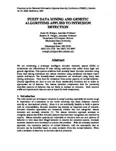
5 Experimental Results In order to evaluate the effectiveness of FARM, we applied it to a real-life database concerning with the agriculture business in mainland China. The database contains data obtained from a survey about the economic situations of 280 villages in 1992. The scope includes production process, organizational structure, and working capital, etc. This database consists of 280 records and each record is characterized by 167 attributes. There are 99.6% of records having missing values in at least one of the attributes. As an illustration, let us consider attribute Capital-oftransportation in detail. We define the linguistic terms Very-low, Low, Moderate, High, Very-high, and Extremelyhigh for Capital-of-transportation (Fig. 7). Very-low
Low Moderate High
Very-high
Extremely-high
Degree of membership
1
0 0.01
0.1
1
10 100 Capital-of-transportation
1000
10000
Fig. 7. Definition of linguistic terms for attribute Capital-of-transportation. Using the linguistic terms described in Section 3.1, we applied FARM to the database. Among the fuzzy association rules discovered by FARM, the following rules are particularly interesting. Capital-of-transportation = High [1.53] Investment-in-construction = Very-high Capital-of-agriculture = Very-high Capital-of-transportation = High [1.17] Investment-in-construction = Very-high ∧ Capital-of-agriculture = High Capital-of-transportation = High [3.51] �
�
�
6
The first one says that very high investment in construction tends to introduce high capital of transportation whereas the second one says that very high capital of agriculture is associated with high capital of transportation. Based on these two rules, it is reasonable that both of these two factors is related to high capital of transportation. It is exactly what the third rule says. The fact that the weight of evidence of the third rule is substantially greater than the weight of evidence of the first and the second rules means that the capital of transportation is more likely to be high when both the investment in construction and the capital of agriculture are very high at the same time. Let us consider the following fuzzy association rule as well. Income-of-industry = Very-low ∧ Capital-of-commerce-and-food-&-beverage = Very-low ∧ Capital-of-commerce-and-food-&-beverage-(self) = Very-low Capital-of-transportation = Moderate [-4.80] �
This rule states that there will not even be moderate capital of transportation when the income of industry and the overall and the self used capital of commerce and food & beverage are very low. This rule is an example of negative association rules. It should be noted that existing algorithms (e.g. [1, 11]) are unable to discover negative associations. The ability of FARM to mine negative association rules is another unique feature of it. Among the attributes in the database, one of them, called Capital-of-transportation, is identified as the class attribute for further experimentation. Of the 280 records, 220 are randomly selected for training and the others are used for testing. The attribute Capital-of-transportation is quantitative and the predictions on this attribute are therefore of quantitative values. Unfortunately, many data mining techniques (e.g. [1, 11]) which can only classify a record into appropriate category are unable to give quantitative values as predictions. As a result, they are not readily applicable to this task. On the contrary, by representing attribute Capital-of-transportation with a set of linguistic terms, FARM is able to produce predictions which are of quantitative values. The root mean squared error calculated by (11) over the class attribute Capital-of-transportation for the database is equal to 4.5%. In other words, the predictions produced by our algorithm deviated from the target values by 4.5% in average. 6 Conclusions We presented a novel algorithm, called FARM, which employs linguistic terms to represent the revealed regularities and exceptions in this paper. The definition of linguistic terms is based on fuzzy set theory and hence we call the rules having these terms fuzzy association rules. Unlike other algorithms which discover association rules based on the use of some user supplied threshold such as minimum support and minimum confidence, FARM employs adjusted difference analysis to identify interesting associations among attributes without using any user supplied thresholds. FARM also has unique features that it is able to discover both positive and negative associations and it uses a confidence measure, called weight of evidence, to represent the uncertainty associated with the fuzzy association rules. Furthermore, FARM has another unique feature that quantitative values can be inferred from fuzzy association rules. This allows interesting associations between different quantitative values to be revealed. References [1] R. Agrawal, T. Imielinski, and A. Swami, “Mining Association Rules between Sets of Items in Large Databases,” in Proc. of the ACM SIGMOD Int’l Conf., Washington D.C., May 1993, pp. 207-216. [2] W.-H. Au and K.C.C. Chan, “An Effective Algorithm for Discovering Fuzzy Rules in Relational Databases,” in Proc. of the 1998 IEEE Int’l Conf. on Fuzzy Systems, Anchorage, Alaska, May 1998, pp. 1314-1319. [3] K.C.C. Chan and W.-H. Au, “An Effective Algorithm for Mining Interesting Quantitative Association Rules,” in Proc. of the 12th ACM Symp. on Applied Computing, San Jose, CA, Feb. 1997, pp. 88-90. [4] K.C.C. Chan and W.-H. Au, “Mining Fuzzy Association Rules,” in Proc. of the 6th ACM Int’l Conf. on Information and Knowledge Management, Las Vegas, Nevada, Nov. 1997, pp. 209-215. [5] K.C.C. Chan and A.K.C. Wong, “A Statistical Technique for Extracting Classificatory Knowledge from Databases,” in [10], pp. 107-123. [6] U.M. Fayyad, G. Piatetsky-Shapiro, P. Smyth, and R. Uthurusamy (Eds.), Advances in Knowledge Discovery and Data Mining, AAAI/MIT Press, 1996. [7] D.E. Goldberg, Genetic Algorithms in Search, Optimization, and Machine Learning, Addison-Wesley, 1989. [8] K. Hirota and W. Pedrycz, “Linguistic Data Mining and Fuzzy Modelling,” in Proc. of the 5th IEEE Int’l Conf. on Fuzzy Systems, New Orleans, LA, Sep. 1996, pp. 1488-1492. [9] D.H. Lee and M.H. Kim, “Database Summarization Using Fuzzy ISA Hierarchies,” IEEE Trans. on Systems, Man, and Cybernetics – Part B: Cybernetics, vol. 27, no. 4, pp. 671-680, Aug. 1997. [10] G. Piatetsky-Shapiro and W.J. Frawley (Eds.), Knowledge Discovery in Databases, AAAI/MIT Press, 1991. [11] R. Srikant and R. Agrawal, “Mining Quantitative Association Rules in Large Relational Tables,” in Proc. of the ACM SIGMOD Int’l Conf., Monreal, Canada, June 1996, pp. 1-12. [12] R.R. Yager, “On Linguistic Summaries of Data,” in [10], pp. 347-363.
7