largest utilities in California, Pacific Gas and Electric Co. and Southern California. Edison Co., in ... California, excluding San Diego County. This includes all cars ...
A Demand Forecasting System for Clean-Fuel Vehicles
David Brownstone Department of Economics University of California at Irvine Irvine, CA 92717
David S. Bunch Graduate School of Management University of California at Davis Davis, CA 95616
Thomas F. Golob Institute of Transportation Studies University of California at Irvine Irvine, CA 92717
Working Paper May 1994 presented at the OECD conference on ÒFuel Efficient and Clean Motor Vehicles,Ó Mexico City
UCTC No. 221 The University of California Transportation Center University of California at Berkeley
The University of California Transportation Center The University of California Transportation Center (UCTC) is one of ten regional units mandated by Congress and established in Fall 1988 to support research, education, and training in surface transportation. The UC Center serves federal Region IX and is supported by matching grants from the U.S. Department of Transportation, the California Department of Transportation (Caltrans), and the University. Based on the Berkeley Campus, UCTC draws upon existing capabilities and resources of the Institutes of Transportation Studies at Berkeley, Davis, Irvine, and Los Angeles; the Institute of Urban and Regional Development at Berkeley; and several academic departments at the Berkeley, Davis, Irvine, and Los Angeles campuses. Faculty and students on other University of California campuses may participate in
Center activities. Researchers at other universities within the region also have opportunities to collaborate with UC faculty on selected studies. UCTCÕs educational and research programs are focused on strategic planning for improving metropolitan accessibility, with emphasis on the special conditions in Region IX. Particular attention is directed to strategies for using transportation as an instrument of economic development, while also accommodating to the regionÕs persistent expansion and while maintaining and enhancing the quality of life there. The Center distributes reports on its research in working papers, monographs, and in reprints of published articles. It also publishes Access, a magazine presenting summaries of selected studies. For a list of publications in print, write to the address below.
University of California Transportation Center
108 Naval Architecture Building Berkeley, California 94720 Tel: 510/643-7378 FAX: 510/643-5456
The contents of this report reflect the views of the author who is responsible for the facts and accuracy of the data presented herein. The contents do not necessarily reflect the official views or policies of the State of California or the U.S. Department of Transportation. This report does not constitute a standard, specification, or regulation.
A Demand Forecasting System for Clean-Fuel Vehicles David Brownstone Department of Economics University of California, Irvine David S. Bunch Graduate School of Management University of California, Davis Thomas F. Golob Institute of Transportation Studies University of California, Irvine
ABSTRACT This paper describes an ongoing project to develop a demand forecasting model for clean-fuel vehicles in California. Large-scale surveys of both households and commercial fleet operators have been carried out. These data are being used to calibrate a new micro-simulation based vehicle demand forecasting system. Based on pre-specified attributes of future vehicles (including specified clean-fueled vehicle incentives), the system will produce annual forecasts of new and used vehicle demand by type of vehicle and geographic region. The system will also forecast annual vehicle miles traveled for all vehicles and recharging demand by time of day for electric vehicles. These results are potentially useful to utility companies in their demand-side management planning, to public agencies in their evaluation incentive schemes, and to manufacturers faced with designing and marketing clean-fuel vehicles.
1.
Introduction
Manufacturers and government agencies interested in promoting clean-fuel vehicles need to know how demand is affected by attributes that distinguish these vehicles from conventional gasoline or diesel vehicles. Such attributes include: range between refueling, overnight recharging requirements (electric), the potential availability of at-home refueling (compressed natural gas), the availability of refueling and opportunity recharging stations, vehicle performance levels, cargo carrying capacity, and capital and operating cost differences compared to conventional-fuel vehicles. It is also important to establish the extent to which consumers are attracted to vehicles that have reduced tailpipe emissions, as well as the effectiveness of various proposed incentives designed to promote sales and use of clean-fuel vehicles. This is especially important in states like California,
where stringent vehicle emission standards have been adopted or proposed. This year, the California Air Resources Board (CARB) will require manufacturers to produce and sell about 150,000 low-emission vehicles (about 10 percent of the stateÕs annual new car fleet). All new cars sold in the state will be required to emit 80 percent less hydrocarbons by the year 2000, and 50 to 75 percent less carbon monoxide and nitrogen oxide. CARB has also mandated the production and sale of zero-emission (electric) vehicles, beginning with 2 percent of annual car sales in 1998 and increasing to 10 percent in 2003. Because of uncertainty over consumer response to these mandates, the two largest utilities in California, Pacific Gas and Electric Co. and Southern California Edison Co., in cooperation with the California Energy Commission, are sponsoring a project to develop a dynamic demand forecasting model for clean-fuel vehicles in California. The model development work is being carried out by the University of CaliforniaÕs Institute of Transportation Studies at Irvine and Davis. This paper briefly describes the requirements and structure of the model and the new largescale surveys required to calibrate the model. Finally, we report some preliminary empirical results. This research builds upon previous efforts to provide quantitative estimates of demand for electric and alternative fuel vehicles. These estimates are useful for evaluating incentive polices, vehicle design and marketing strategies, and fuel demand management. It is not possible to discuss all of these precursor studies here, but the list is headed by the following: Beggs and Cardell, 1980; Beggs, Cardell and Hausman, 1981; Hensher, 1982; Calfee, 1985; Greene, 1989, 1990; and Train, 1980.
2.
Model Requirements and Structure
2.1. Requirements The forecasting model is being designed to forecast demand for all types of vehicles subject to clean air mandates for each of 79 urbanized regions in California, excluding San Diego County. This includes all cars and light duty trucks (pickup trucks, vans, and sport utility vehicles), as well as medium duty trucks up to 14,000 pounds gross vehicle weight. The geographic regions are defined to be consistent with utility company service planning areas. The model will also forecast fuel usage for each type of vehicle in each region. To determine the impact of electric vehicle recharging on the electric transmission and distribution system, we will also forecast recharge demand for electric vehicles by time of day. Currently, peak electricity demand in California occurs during summer afternoons, and minimum demands occur between midnight and 6:00 A.M.
Therefore, electric vehicle recharging will be much cheaper and less polluting if it takes place during late night hours when electricity is generated by hydroelectric and other clean baseline plants. All conventional-fuel and clean-fuel vehicle types that are anticipated to be available during the forecast period will be included in the model. All makes and models of vehicles will be grouped into relatively homogeneous classes with similar attributes, such as emission levels. Our initial model will use 14 personal vehicle classes (7 car classes and 7 light truck classes), with each class further subdivided into 10 model-year vintage subclasses. The commercial fleet submodel will contain a medium-duty truck class in addition to all of these light truck and car classes, all broken down into similar model-year vintage subclasses. Since we are primarily interested in forecasting the demand for new types of vehicles, the model must be able to forecast the technology adoption process. This requirement rules out the classic static vehicle demand models, such as Train (1986). Our model must produce a separate forecast for the each period, and the next periodÕs forecast must depend on all the previous forecasts. Although we need to account for all vehicles in the California market, we do not explicitly model the behavior of state and federal government and rental car fleets. The flow of used vehicles into the used vehicle and scrappage market is determined by separate simple models estimated from two years of linked vehicle registration files. 2.2. Basic Structure The basic structure of the model system starts from the current condition and forecasts vehicle transactions, which then determine the vehicle stock for the next period. The vehicle stock for the baseline year, 1994, is determined by a current census of vehicle registrations augmented by large scale surveys of household and fleet behavior. This structure is similar to HensherÕs (1992) system. Hensher represents the household population by a relatively small number of ÒsyntheticÓ households, while we use a large sample of actual households and fleets. Our microsimulation approach requires more computation, but should be more accurate. The two main models in our system, the personal and fleet vehicle demand models, are both transactions models: they predict whether a vehicle transaction will occur during the current period and what type of transaction it will be. The inputs to these models are the current characteristics of the household (or fleet) and the current vehicle inventory and utilization. Since vehicle type decisions are discrete, the models can only provide probabilities that a particular household or firm will
choose a particular type of vehicle. Forecasting a particular choice from these models requires simulating an actual choice, which introduces some random noise into the forecasting process. Fortunately, the effect of this randomness disappears when forecasts for individual households or fleets are aggregated to predict market demand. The predicted changes in vehicle holdings and utilization are then combined with initial holdings to forecast vehicle stocks for the next period. Since our transactions models are estimated using standard econometric techniques, the parameters are subject to estimation error. The effects of these errors on the resulting forecasts will be measured by a ÒbootstrappingÓ process (Efron and Tibshirani, 1993). A number of different forecasts will be generated using different parameter values chosen to represent the parameter estimation uncertainty. The resulting spread of forecasts will generate confidence regions for our forecasts. 2.3. Exogenous Inputs The key inputs to our forecasting system are vehicle technology, fuel prices, fuel infrastructure, and incentives. Vehicle technology includes all attributes of vehicles which will become available in the future, including fuel type, refueling or recharging range, price, operating costs, vehicle tailpipe emissions, payload, and performance. Although it is relatively easy to forecast these attributes two to three years ahead, it is very difficult to predict the state of new technology ten or more years ahead. Forecasts from the model system crucially depend on future vehicle technology, and users of the model system will need to continually update this information as time progresses. Since the model produces forecasts for each year, it is also important to forecast when new technology vehicles will be introduced. Finally, the model system assumes that manufacturers are willing to provide as many vehicles as demanded at the forecast vehicle price. Fuel prices are another exogenous input to the model system. Although these are typically very difficult to forecast, we only need accurate forecasts of relative fuel prices. The prices of three of the fuels considered in our model -- gasoline, compressed natural gas, and electricity -- have tended to move together with the price of crude oil during the past decade. However, if crude oil prices start to rise substantially, then the off-peak electricity price may diverge from recent patterns since in California off-peak electricity is primarily generated by hydroelectric power. Fuel infrastructure describes the availability of alternative clean fuels. For compressed natural gas and methanol this is described by the percentage of existing service stations that sell the fuel. The electricity fuel infrastructure also
includes the types of places (e.g. shopping centers, airports, etc.) where Òopportunity chargingÓ is available. The final set of exogenous inputs are incentives for purchasing clean-fuel vehicles. Many proposed incentives (such as, sales tax and vehicle registration fee subsidies) simply lower the capital and/or operating costs of these vehicles, s o the effects of these incentives can be modeled by changing the appropriate cost variables in the vehicle technology section. Other proposed incentives, such as free parking, solo driver access to high-occupancy vehicle (carpool) lanes, or extended vehicle warranties, do not directly affect vehicle technology. Our surveys are being designed so that both the personal and fleet demand submodels can be sensitive to such incentives, so that the forecasting system can be used to evaluate a wide range of proposed incentive policies. 2.4. Used Car and Scrappage submodel The bi-directional arrows between the used vehicle market and demand submodels in Figure 1 indicate that the model system will internally set used car prices so that the demands for used cars forecast by the submodels equals the predicted number of used cars sold by the submodels. This price equilibration will be performed separately for small groups of vehicle type-vintage classes. Therefore, one important feature of our model system is that it will provide estimates of used prices for clean-fuel vehicles. Our approach requires that the used vehicle market in California is closed, or that used-vehicle price differences do not cause people to move vehicles in or out of the state. This assumption is reasonable given CaliforniaÕs geography: the main urban areas are far away from urban areas in neighboring states. Although our personal vehicle and fleet demand submodels exclude rental and state and federal fleets, these fleets are an important source of vehicles entering the used market. At this time, it appears that rental fleets will be excluded from all clean-fuel vehicle mandates, so we will model their behavior as fixed throughout the forecast period. Specifically we will assume that rental fleets purchase and sell the same type and number of vehicles as they did in 1993-1994. For political reasons, state and federal fleets will need to meet clean-fuel vehicle mandates. We will therefore assume that they purchase enough vehicles to meet these mandates in the lowest-cost fashion. We will also assume that these fleets continue to follow the same vehicle sales and scrappage policies as in 1993-1994. Clearly our rental and government fleets ÒmodelsÓ could be considerably improved. Unfortunately, the required data collection is beyond the scope of the current project.
2.5. Personal Vehicle Submodel The personal vehicle submodel is the most complicated part of our modeling system. It consists of a number of linked models shown schematically in Figure 2. The initial current vehicle holdings and household structure are taken from the personal vehicle survey described in Section 3.3. Box A in Figure 2 represents a series of models which age each household, and simulate births, deaths, divorces, children leaving home, etc. Once the new household structure is determined, other models in Box A determine the householdÕs income and employment status.
Figure 1: Schematic Representation of Model System
Current Vehicle Stock
Personal Vehicle Demand M odel
Exogenous: Vehicle Technology, Fuel Prices, and Incentives
Fleet Vehicle Demand M odel Rental and Government Fleet Sales
Demand for new personal vehicles, utilization of current vehicle stock
Used Vehicle M arket and Scrappage
Vehicle Stock Next Period
Demand for new fleet vehicles, utilization of current vehicle stock
Figure 2: Personal Vehicle Submodel
Current Vehicle Holdings
Current Household Structure
A. Update Household Sociodemographic Structure
B. Transaction this period? Yes
C. Household Vehicle Transaction M odel
Update Household Vehicle Holdings
No
D. Vehicle Utilization M odel
The dotted line leaving Box A shows that this updated household is used as the starting point for aging the household in the next period. Note that the models in Box A are mostly calibrated from the Panel Study of Income Dynamics (Hill, 1992) because our personal vehicle survey does not track households over a sufficiently long time period to be used as a calibration source. Ellipse B in Figure 2 takes the updated household and current (aged) vehicle holdings as inputs. It then decides whether or not a vehicle transaction takes place during this period. The period length is set at six months, in order to limit the number of transactions per period to one, but model system outputs are given
annually. A vehicle transaction is defined to include: disposing of an existing vehicle, replacing an existing vehicle with another one, or adding a new vehicle to the householdÕs fleet. If the simulation from the transactions model in Ellipse B predicts that a vehicle transaction has taken place, the transaction type model in Box C determines exactly what type of transaction takes place. The householdÕs vehicle holdings are updated accordingly, and these are used as inputs to the vehicle utilization model in Box D as well as starting values for the next periodÕs forecast. The model outputs for each year accumulate the probabilities of all actions to the total numbers of vehicles owned or leased by type and vintage. For new vehicles, this represents market penetration. The utilization model takes the updated vehicle holdings and household structure as inputs. It then predicts the annual vehicle miles traveled for each household vehicle. The usage forecasts are then converted to fuel demand by using average miles per gallon for liquid fuels and miles per equivalent gallons for non-liquid fuels. For electric vehicles, the utilization model also predicts the frequency of recharging at different times of day. 2.6. Fleet Vehicle Submodel The fleet vehicle submodel is similar to the personal vehicle submodel depicted in Figure 2, except that the firm analog to sociodemographic updating in Box A is replaced by simple reweighting. We assume that the firms in our fleet sample remain the same throughout the forecast period except for their vehicle transactions and utilization. Changes in industry structure are accommodated by changing the weights assigned to each firm in our sample to match external forecasts of employment by business sector for each region. The other difference from the personal vehicle submodel is that the transaction model for fleets doesnÕt forecast the results of one vehicle transaction. Instead it forecasts the changes in the fleetÕs composition based on the current fleet holdings and type of business.
3.
Data Requirements
This section describes the data required to calibrate the models described in Section 2. Since we are concerned with the demand for a new product that does not yet, we must ask respondents to make choices among hypothetical vehicles. These Òstated preferenceÓ questions (Louviere, 1988) have been successfully used in a pilot study of consumer preferences for alternative fuel vehicles (Bunch, at al., 1993; Golob, at al. 1993). This pilot study, sponsored by the California
Energy Commission, confirmed that information about attribute trade-offs gained through our Òstated preferenceÓ method are consistent with results of previous studies of actual vehicle purchase behavior (e.g., Train, 1980, 1986; Hensher, 1992). Stated preference questionnaires require that respondents receive different hypothetical vehicles according to a pre-specified experimental design. The questionnaires must also contain enough background information so that respondents can fairly evaluate the hypothetical vehicles. In addition to stated preference questions, we must also ask extensive questions about respondentsÕ existing vehicle stock and utilization. The remainder of this section gives more detail about the three main data sets used to calibrate our models. 3.1. Personal Vehicle Panel Survey The first wave of our personal vehicle panel survey was carried out in June and July, 1993. The sample was identified using pure random digit dialing and was geographically stratified into 79 areas covering most of the urbanized area of California. 7,387 households completed the initial computer-aided telephone interview (CATI). This initial CATI interview collected information on: household structure, vehicle inventory, housing characteristics, basic employment and commuting for all adults, and the next vehicle transaction. The data from the initial CATI interview were used to produce a customized mailout questionnaire for each sampled household. This questionnaire asked more detailed questions about each household memberÕs commuting and vehicle usage, including information about sharing vehicles in multiple-vehicle and multipledriver households. The mail-out questionnaire also contained two Òstated preferenceÓ experiments for each household. Each of these experiments described three hypothetical vehicles, from which the households were asked to choose their preferred vehicle. These hypothetical vehicles included both clean-fuel and gasoline vehicles, and the body types and prices were customized to be similar (but not identical) to the householdÕs description of their next intended vehicle purchase. After the households received the mail-out questionnaires, they were again contacted for a final CATI interview. This interview collected all the responses to the mail-out questions. Additional questions about the householdÕs attitudes towards clean-fuel vehicles were also included in this interview. 4747 households completed all phases described above, and the information from these households is the basis for the preliminary results described in Section 4.
The second wave of the personal vehicle survey is scheduled to begin in May, 1994. The panel will be refreshed with at least an additional 1000 households to measure the effects of non-random panel attrition and conditioning. This second wave interview will also be a hybrid CATI - mail-out - CATI survey. The second wave Òstated preferenceÓ task will involve more hypothetical vehicles and will be more focused on vehicle transactions based on the householdÕs current vehicle holdings. We will also collect information on all changes in the householdÕs structure, vehicle holdings, and housing, and we will track and attempt to interview all household members who were in the household at the time of our first wave interview. 3.2. Fleet Survey The first task in surveying commercial and local government (city, county and regional) fleet operators was to establish a comprehensive list of fleets from which a survey sample could be drawn and a universe can be established. Many small to medium size fleet operators are not currently registered in fleet databases available from fleet managersÕ associations, governmental agencies, or commercial market research firms. Moreover, these databases are not generally up to date on the number and type of vehicles operated in a given fleet. Consequently, a comprehensive list of potential fleets was obtained from the 26.5 million records of the California Department of Motor Vehicles registration file. A knowledge-based pseudo artificial intelligence system was developed to match and combine all vehicle registrations with a high probability of being the same company or individual at the same site, taking into account differences in registrations due to abbreviations and spelling. Most clean-air mandates target fleets sites with 10 or more vehicles, so all potential sites with 5 or more registrations were investigated because it is still possible that registration sites will be fragmented into two or more components based on unresolved differences in names or addresses. Since substantial numbers of households own or lease five or more vehicles, and many households even own 10 or more vehicles, a knowledge-based system using rules and predicate logic for conflict resolution was developed to separate households from businesses. A sample was then drawn from the identified registration sites, and survey results are used to factor the total list of registration sites in order to estimate the universe of commercial and local government fleet sites. The survey of 2,000 fleet sites was conducted as a combined CATI and mail-back questionnaire. The CATI portion of the survey established the fleet inventory, business functions, and gathered data on multi-site fleet operations. In the customized mail-back questionnaire, fleet operators provided detailed operation
and acquisition data on up to two selected types of vehicles currently in their fleets. In the mail-out SP tasks, the operators chose future fleets of the selected types from among hypothetical conventional-fuel and alternative-fuel vehicles, and they allocated the chosen vehicles to the tasks typically performed by the fleet. There were also questions concerning organizational decision making and opinions about alternative-fuel vehicles. 3.3. Census of Vehicle Registrations The 1993 California Department of Motor Vehicles registrations are used to generate a fleet universe and sample are also crucial for establishing the initial number of vehicles by type/vintage class for each region. We will obtain another list of vehicle registrations for 1994, which will be linked back to the same vehicles if they were registered in 1993. Since the vehicle registration list records the date and odometer readings when vehicles are transacted or scrapped, we will use these linked lists to learn about the purchase and disposal patterns of rental and government fleets. More generally, we will also use these linked lists to model vehicle scrappage decisions. The separation of registrations into personal-use and fleet vehicles was accomplished using probabilities developed from algorithms based on results from both the fleet and personal vehicle surveys. Company cars which go home with employees were divided into personal-use and fleet vehicles depending upon who makes the decision regarding the type of vehicle to be purchased or leased; questions to determine this were included in the surveys. CD-ROM drives were used to accommodate the large registration data files.
4.
Preliminary Results
4.1. Descriptive results of personal vehicle survey The 4747 households that successfully completed the mail-out portion of wave one of the personal vehicle survey in 1993 represent a 66% response rate among the households that completed the initial CATI survey. A comparison with Census data reveals that the sample is slightly biased toward home-owning larger households with higher incomes, and weights are being applied to balance the sample to the known population. Importantly, 18% of the surveyed households had more than one phone number, and 7% of the households shared a phone with at least one other household. These are important statistics in weighting the households to account for their probability of being selected in a random-digitdialing sample.
Regarding vehicle ownership and use, 80% of the households in the sample had exactly one driver per vehicle, proving that, in California, the number of drivers is the most important determinant of the vehicle ownership level. For two vehicle households, a little over one-third of the vehicles are driven 10,000 miles per year or less, a third are driven 10,000 - 15,000 miles per year, and almost a third are driven more than 15,000 miles per year. Regarding long trips, 54% of these vehicles are driven on trips of 100 miles or more six or fewer times per year. Another potential problem is whether households can accommodate a limitedrange clean-fuel vehicle that requires home recharging. Our survey results show that 16% of all households commute less than 30 miles per day round trip and also have a private garage or carport with electric service. 20% of all households commute less than 60 miles per day round trip and also have a private garage or carport with electric service. Finally, 21% commute less than 120 miles per day round trip and also have a private garage or carport with natural gas service nearby. 4.2. Tradeoffs Between Hypothetical Vehicles The data from the hypothetical choices have been analyzed using multinomial logit and nested multinomial logit models (see Ben-Akiva and Lerman, 1985) to examine the relative importance of the various attributes discussed earlier. Preliminary analyses have been performed in which the effect of changing an attribute is measured in terms of its tradeoff versus vehicle purchase price. For example, if the refueling range of a vehicle is decreased, how much must the purchase price be lowered for the "average" consumer to remain "indifferent"? In this analysis, "indifferent" means that the purchase probability for the vehicle would remain unchanged. Suppose we were to take a typical gasoline vehicle and modify its attributes to make it more like an alternative fuel vehicle. We will consider the separate effect of a 50% change in each attribute level, and define "sensitivity" based on the magnitude of the purchase price tradeoff. Consider a "typical" vehicle with a 300 mile range, 6 cents per mile fuel operating cost (20 mpg with gasoline costing $1.20 per gallon), and emissions typical of 1993 gasoline cars. Gasoline is available at all stations. We separately consider the effect of changing range to 150 miles, operating cost to 3 cents per mile, reducing emissions by 50%, and reducing fuel availability by 50%. On this basis, the most sensitive attribute is vehicle range, followed by operating cost, emissions, and fuel availability, respectively. The approximate tradeoff values are: ($7,500), $4,000, $3,500, and ($500), respectively (where parenthesis indicate negative values). It is important to know, however, that preferences for these attributes exhibit varying
degrees of nonlinearity outside the limits considered here. Thus, any analysis should be conducted carefully on a case-by-case basis. This example is presented to indicate the overall nature of our findings. 4.3.
Comparison Between Hypothetical and Observed Vehicle Choice Tradeoffs One possible problem with hypothetical choices made in response to stated preference questions is that respondents may not make the same choices in a realworld setting. Unfortunately, the stated preference study is required because most of the tradeoffs are not available using current vehicles. However, we can compare operating cost tradeoffs between stated preference results and observed vehicle choice behavior. To measure the tradeoffs from observed vehicle choice behavior, we fit a vehicle holdings model very similar to TrainÕs (1986) model. We estimated that onevehicle households with annual incomes less than $30,000 are indifferent between a one cent per mile increase in fuel costs and a $1340 (with a standard error of $830) decrease in vehicle price, and one vehicle households with annual incomes greater than or equal to $30,000 are indifferent between a one cent per mile increase in fuel costs and a $2750 decrease in vehicle price (with a standard error of $4480). Note that these estimates are very close to TrainÕs figures of $1688 and $2268 based on a smaller national sample in 1978. These observed vehicle tradeoffs are also very similar to the $1333 obtained just using tradeoffs between hypothetical vehicles in the stated preference choice experiments. While this single number does not prove that all of our stated preference results will be consistent with observed behavior when real clean-fuel vehicles are available, it is nevertheless encouraging.
5.
Conclusions
The modeling system described in this paper will be capable of analyzing most of the proposed policies for stimulating the demand for clean-fuel vehicles. The system can also be used by vehicle manufacturers to help gauge the demand for various types and configurations of clean-fuel vehicles. Although the key models in the system will be calibrated from new surveys, it will be necessary to undertake additional survey work to validate and extend these models. Our preliminary work suggests that consumersÕ responses to our hypothetical vehicle choice experiments are realistic, but the only proof of this assertion will come when cleanfuel vehicles similar to these hypothetical vehicles are actually offered in the marketplace.
The actual implementation of our modeling system is focused on California since it is the first state to mandate the introduction and sale of clean-fuel vehicles. Other states and countries are also interested in promoting the sale and use of clean-fuel vehicles, and our modeling system should be relatively straightforward to adapt to other regions. This paper has just focused on the demand for clean-fuel vehicles. The main reason for promoting these vehicles is to reduce urban air pollution. A full evaluation of any policy promoting clean-fuel vehicles for reducing pollution must also consider other competing policies such as promoting mass transit use and policies designed to reduce the use of conventional vehicles. This full analysis is beyond the scope of our current efforts, although we hope to extend our model system in the future to make it more useful for evaluating a broader range of pollution and congestion-reducing policies.
6.
Acknowledgments
In addition to our project managers - Ernest Morales (Southern California Edison Co.) and Dan Fitzgerald (Pacific Gas and Electric Co.) - the authors wish to thank their colleagues - Mark Bradley, Ryuichi Kitamura, Stuart Hardy, Jane Torous, Camilla Kazimi, and Weiping Ren - who have all contributed enormously to the work described in this paper. In addition, Gary Occhiuzzo and Mike Jaske of the California Energy Commission, Debbie Brodt of Southern California Edison, and Lisa Cooper of Pacific Gas and Electric have worked diligently on behalf of the project. None of these kind people or their organizations are responsible for any errors or the specific views expressed here.
7.
References
Beggs, S. and S. Cardell (1980). Choice of smallest car by multi-vehicle households and the demand for electric vehicles. Transportation Research, 14A: 389-404. Beggs, S., S. Cardell and J. Hausman (1981). Assessing the potential demand for electric cars. Journal of Econometrics, 16: 1-19. Ben-Akiva, M. and S.R. Lerman (1985). Discrete Choice Analysis: Theory and Application to Travel Demand. MIT Press, Cambridge, MA. Bunch, D.S., M. Bradley, T.F. Golob, R. Kitamura, and G.P. Occhiuzzo (1993). Demand for clean-fuel vehicles in California: A discrete-choice stated preference pilot project. Transportation Research, 27A: 237-253.
Calfee, J.E. (1985). Estimating the demand for electric automobiles using fully disaggregated probabilistic choice analysis. Transportation Research, 19B: 287-302. Efron, B. and R. Tibshirani, 1993. An Introduction to the Bootstrap. Chapman and Hall, New York. Golob, T.F., R. Kitamura, M. Bradley and D.S. Bunch (1993). Predicting the market penetration of electric and clean-fuel vehicles. The Science of the Total Environment, 134: 371-381. Greene, D.L. (1989). Motor fuel choice: An econometric analysis. Transportation Research, 23A: 243-254. Greene, D.L. (1990). Fuel choice for multi-fuel vehicles. Contemporary Policy Issues, 8: 118-137. Hensher, D.A. (1982). Functional measurements, individual preferences and discrete choice modeling: Theory and application. Journal of Econometric Psychology, 2: 323-335. Hensher, D.A. (1992). Dimensions of Automobile Demand. Elsevier, Amsterdam. Hill, M. (1992). The Panel Study of Income Dynamics: A Users Guide. Sage Publications, Newberry Park, CA. Louviere, J. (1988). Conjoint analysis modeling of stated preferences: A review of theory, methods, recent developments and external validity. Journal of Transport Economics and Policy, 12: 93-120. Train, K. (1980). The potential market for non-gasoline-powered vehicles. Transportation Research, 14A: 405-414. Train, K. (1986). Qualitative Choice Analysis. MIT Press, Cambridge, MA.