the simulation model can be interpreted as a deterministic model that approximates stochastic processes such as Rayleigh, log- normal, and Suzuki processes.
318
IEEE TRANSACTIONS ON VEHICULAR TECHNOLOGY, VOL. 45, NO. 2, MAY 1996
inistic Digital Simulatio cesses wi lication t le io
r owe anne
Matthias Patzold, Ulrich Killat, Member, ZEEE, and Frank Laue
bandwidth is much smaller than the coherence bandwidth of the channel, so that a non-frequency-selective channel model is appropriate. Hence, the received signal is simply the transmitted signal multiplied by an appropriate stochastic process, which represents the time-variant characteristics of the channel. Furthermore, we will restrict our attention to urban areas, where the direct-line-of-sight component between the mobile vehicle and the base station is for most of the time completely obstructed by high buildings. In such cases, the signal at the receiver is composed of many independent reflected signal components coming from all directions in the horizontal plane. These signal components can constructively or destructively add to give a received signal that varies randomly in amplitude and phase. The envelope of the received signal is then Rayleigh I. INTRODUCTION distributed and the phase is uniformly distributed over the P to the present day, a number of computer simulation interval 0-2n. If the vehicle moves a small distance, the environment models have been proposed for the simulation of the fadcharacteristics can be considered as approximately constant, ing characteristics of cellular mobile radio channels. Mostly, and therefore, the power of the Rayleigh process can also be the computer simulation models are based on the shaping considered as approximately constant. But for larger distan'ces, of the power spectral density of at least two or more white the environment characteristics are slowly varying, and the Gaussian noise processes by using recursive digital filters. In general, the bandwidth of the shaping filters are extremely power of the Rayleigh process can vary considerably. In this small in comparison with the sampling frequency. In order to case, a Suzuki process [4] models the stochastic process more circumvent numerical difficulties encountered with the design precisely. The Suzuki process is obtained by the multiplication of recursive digital filters having a small bandwidth, one of a Rayleigh process with a log-normal process. The average usually uses linear interpolation techniques for the required duration of fades and the level crossing rate of Suzuki prosampling rate conversion. But in this way, the numerical effort cesses are of great importance and have been investigated in and the transient behavior increases. Recently, generative [51-[71. This paper is organized as follows. First, we will describe channel models based on finite state models, which need lower the Suzuki model in Section 11. For this statistical model we numerical effort than those using digital filters, have been will present in Section I11 an efficient computer simulation proposed [ 11. In this paper, a novel computer simulation model for a land model that can consequently be used for the simulation of mobile radio fading channel that avoids digital filtering as well a land mobile radio channel. Afterwards in Section IV, we as linear interpolation is proposed. Our model is based on describe four completely different methods for the derivation the approximation of filtered white Gaussian noise processes of the simulation model parameters, and we compare in by finite sums of properly weighted sinusoids with equally Section V the performance of these procedures on the basis distributed phases. Although the principle of the method of two quality criteria. Finally, we present in Section VI some presented here can immediately be applied to the design of examples and simulation results in order to demonstrate the frequency-selective channels [2],[ 3 ] , we restrict-for reasons power of the methods derived in this paper. of simplification-our attention to systems, where the signal
Abstract- We present a novel computer simulation model for a land mobile radio channel. The underlying channel model takes for granted non-frequency-selectivefading but considers the effects caused by shadowing. For such a channel model we design a simulation model that is based on an efficient approximation of filtered white Gaussian noise processes by finite sums of properly weighted sinusoids with uniformly distributed phases. In all, four completely different methods for the computation of the coefficients of the simulation model will be introduced. Furthermore, the performance of each procedure will be investigated on the basis of two quality criteria. All the presented methods have in common that the resulting simulation model has a completely determined fading behavior for all time. Therefore, the simulation model can be interpreted as a deterministic model that approximates stochastic processes such as Rayleigh, lognormal, and Suzuki processes.
Manuscript received November 24, 1994; revised May 22, 1995. The authors are with the Department of Digital Communication Systems, Technical University of Hamburg-Harburg, D-21071 Hamburg, Germany. Publisher Item Identifier S 0018-9545(96)00954-1.
11. THESUZUHMODEL
The Suzuki model is a statistical model that has been developed for the land mobile radio channel on the assumption
0018-9545/96$05.00 0 1996 IEEE
-
PATZOLD et ai.: DETERMINISTIC DIGITAL SIMULATION MODEL FOR SUZUKl PROCESSES
that the local mean of the Rayleigh process follows a lognormal statistic and accounts therefore for the effects caused by shadowing. According to [4], a stationary Suzuki process ~ ( tis) a product process of a Rayleigh process E(t) and a log-normal process [ ( t ) ,i.e.
Q ( t= ) E(t) . C(Q
spectral density function S,, ( f ) is of no great inflbence on the statistical properties of the Suzuki process [7]. By applying the inverse Fourier transform on (7), we obtain the autocorrelation function ;rP, ( t )of the Gaussian process p3(t)
(1)
The Rayleigh process E(t) is per definition [SI obtained from the envelope of a narrow-band complex Gaussian (normal) random process P ( t ) = Pl(t) + jPLa(t)
319
Other classes of spectral shaping filters, such as %pole Buttenvorth filters and RC-lowpass filters, have been used in [ 101 and [5], l[6], respectively.
(2)
where p l ( t ) and p 2 ( t ) are uncorrelated real normal processes with zero means E { p i ( t ) } = mi = 0 and identical variances Var{pi(t)} = = r&, i = 1,2. Therefore
vit
(3) is a Rayleigh-distributed random process. The assumption of statistical independence between p1 ( t ) and pz ( t ) does not always meet the real conditions encountered in multipath wave propagation. For that reason, modified Rayleigh processes and thus modified Suzuki processes with a nonzero cross correlation between p1 ( t )and p2(t) have been introduced in [6]. For spectral shaping of the real normal processes p i ( t ) , i = 1,2, the Jakes power spectral density function [9]
111. THESIMULATION MODEL In the previous section, we have seen that the realization of a Suzuki process is based on the generation of three uncorrelated filtered white Gaussian noise processes pz(t),i= 1,2,3. As already mentioned, our simulation model presented in this paper avoids digital filtering, as well as linear interpolation, for the realization of the Gaussian processes p, ( t ) i, = 1 , 2 , 3 . Instead of this, we make use of the fact that each Gaussian process p z ( t )can be approximated by a finite sum of properly weighted sinusoids with uniformly distributed phases [l 11. In the following, we denote the corresponding approximated versions d p z ( t )by fiz(t),and we write N%
bz(t) =
+ @z,n),
cz,n cos(2Tfz,nt
i = 1 , 2 , 3 (9)
n=l
has widely been accepted for cellular land mobile channels, where fmax is called the maximum Doppler frequency. The mean power of p i ( t ) is given by JPmm SPs(f)df = ~7;~. The inverse Fourier transform of (4) gives us for i = 1 , 2 the following identical autocorrelation functions (acf)
(5) where Jo(.) denotes the zeroth order Bessel function of the first kind. The log-normal process [ ( t ) is generated from a further real Gaussian process p3(t) with zero mean m3 = 0 and unit variance v& = 1 according to
[ ( t )= p + w 3 ( t )
(6)
where the parameters m and s are used to transform m3 and v;, to the actual mean and variance, respectively. The real Gaussian process p3(t) is uncorrelated with the complex Gaussian process p ( t ) as defined by (2). For the spectral shaping of the real normal process p3(t), we have assumed the following Gaussian power spectral density function (7) where vc is related to the 3-dB cutoff frequency f c according to f c = acJ27n2. In general, the 3 - d ~cutoff frequency f c is much smaller than the maximum Doppler frequency fmax, say f c = f m a x / ~ , where IC >> 1. For values of K larger than 10, the parameter IC itself as well as the shape of the power
where N, designates the number of sinusoids of the ith process, is named the Doppler coefficient, which represents a real weighting factor of the nth sinusoid, f Z , , is called the discrete Doppler frequency, and @z,n designates a uniformly distributed random phase variable in the interval [0,27r) that will be denoted as Doppler phase. To make our formulas less bulky, we have dropped an index d for all of these quantities, which would remind one that they refer to Doppler frequencies, phases, and coefficients. For a further understanding of the contents of the paper, it is important to realize that a simulation of the approximated Gaussian processes fi,(t), i = 1 , 2 , 3 , requires a computation of the model parameters c ~ ,fZ,,,~ , and during the simulation set up phase. Aftenvards-during the simulation run phase-these parameters are kept constant. Often, diverse simulation runs are desired without changing the statistics of ii,(t). Then, only the ]parameters c , , and ~ fZ,, have to be precomputed and kept constant, while the random phases are generated for each simulation run. Let us assume that the parameters of the simulation model are determined by one of the four methods described in the next section. Hence, all the model parameters introduced in (9) are known quantities, and we can consider ,Gz ( t ) as a deterministic function that approximates the stochastic process p z ( t ) for i = 1 , 2 , 3 . Consequently, the overall simulation model is also a deterministic model that can Ibe used for the approximation and simulation of stochastic processes such as Rayleigh processes ( ( t ) ,log-normal ) . 1 shows the processes =E e, * t 0)
................................................................................................................
’I.
-
Log normal Process .............................................................................................................. ...
................................................................................................................. Fig. 1. Structure of the simulation system.
channel model is predestinated for computer simulations and can easily be obtained by substituting the time variable t by t = k T , where T denotes the sampling interval and k is a natural number. If the parameters of the simulation system are known quantities, analytical expressions can be stated for the autocorrelation function Fpz(t)of (9), as well as for the * which corresponding power spectral density function j P (f), are given by
n=l
quired) if fZ,, # f 3 , m , but they are correlated if f z , n = fJ,m for all n = 1,2,..-,Nz and m = 1 , 2 , . . . , N ,. One special case is of interest, where the Gaussian processes 1-11 ( t )and 1-12 ( t )are correlated and a cross-correlation function ~ ~ ~ meeting , ~ ~the( real t conditions ) can be established [6], [7].For such cases, a cross correlation between the approximated Gaussian processes fil(t) and ,G2(t)of the simulation model can easily be obtained by considering c, = C 1 , n = C Z , n , f n = f ~ =, f ~~ ,and ~ ,0, = 0 1 , = ~ 02,, for all n = 1, 2 , . . . , N = N1 = N2. Hence, the complex process fi(t) = fil(t)+j,&(t) can be written as
+
“ N
N,
?[S(S
Sp%( f )=
-
fi,n>+ ~ (+ ff z , n ) l
(lob)
n=l
for all i = 1 , 2 , 3 , respectively. In the next section, we will show that the set of discrete Doppler frequencies and the corresponding set of Doppler coefficients { c ~ , ~can } be actually determined in such a way that the power spectral (f)of the approximated Gaussian processes fiz(t) densities Sp% are approximated versions of the ideal power spectral density functions S , % ( f ) ,as defined by (4) for i = 1 , 2 and (7) for i = 3. With regard to (9), we see that for i # j , the approximated Gaussian processes fiZ(t)and & ( t ) are uncorrelated (as re-
fi(t)=
Cne3(2Tfnt+w
(11)
n=l
and the cross-correlation function of by ?pl,p,, ( t ) ,is given by
fi1
( t )and fi2(t), denoted
) -? P I ,P2 (4. with TIp1,p2(0)= 0 and ? p l , P 2 ( - t= We remark that methods for the computation of { c ~ , ~ } and { f z , n } can be derived such that ( t ) and ? p a , p j( t )are simultaneously approximated versions of the desired functions r I L I ( t )and T ~ % ( t ), ,respectively. ~ ~ But this problem is beyond
321
PA'IZOLD et al.: DETERMINISTIC DIGITAL SIMULATION MODEL FOR SUZUKI PROCESSES
the scope of the paper. Here, we neglect the influence of a correlation between ,u,(t) and ,ug(t)on the channel statistics, and we restrict our investigations only to an approximation of the autocorrelation function r,%( t ) and the corresponding power spectral density function S,%( f ) .
Iv. COMPUTATION METHODSFOR THE PARAMETERS OF THE SIMULATION MODEL In this section, we consider the computation of the simulation model parameters { c , , ~ } , {f,,n}, and as introduced by (9). Altogether, we present four different methods for the determination of the Doppler coefficients {+} and the corresponding discrete Doppler frequencies { fz,n}. The procedures will be named by method of equal distances, method of equal areas, Monte Carlo method, and mean-square-error method. All the methods are quite different, but nevertheless they have in common that the resulting power spectral density function gPt( f ) [see (lob)] is always an approximated version of the desired power spectral density function S,,(f) as given by (4) and (7) for i = 1 , 2 and i = 3 , respectively. The computation of the Doppler phase variables {E&} is independent of the procedures described below and has to be ensued by means of a random generator having a uniform distribution over [072.rr).We notice that in this case {Oi,,} has no influence on the statistical properties (level crossing rate and average duration of fades) of the approximated processes f i Z ( t ) ,i = 1 , 2 , 3 , but various realizations of k,(t), and therefore various processes ( ( t )and ( ( t )can be obtained for the same sets of { f z , n } and { c ~ , ~by} computing different sets of the Doppler phase variables {Oz,n}. A. Method of Equal Distances (MED)
The characteristic of the method of equal distances (MED) is such that the difference between two adjacent discrete Doppler frequencies is equidistant [ 121. This property is achieved by defining the discrete Doppler frequencies f i , n as follows fi,n :=
%(2n - l ) ,
n = 1 , 2 , . . . ,N,
L
(13)
where
specifies the difference between two adjacent discrete Doppler frequencies of the ith process j&(t),i = 1 , 2 , 3 . are computed by considering The Doppler coefficients the interval
Ii,,:=
if.,- -+, A
-
fi,n
+ nf.) , 2
r~
= 1,2,
for all n = 1 , 2 , . . . , N z and i = 1 , 2 , 3 . In view of the two different types of power spectral densities considered in this paper, wt: adopt the MED to the Jakes power spectral density and the Gaussian power spectral density. 1)Jakes Power Spectral Density: The frequency regions of the Jakes power spectral density functions S,, ( f ) and S,, ( f ) [see (4)] are limited to If1 < fmax. Therefore, a suitable quantity of the difference between two adjacent discrete Doppler frequencies A, is given by A, = fmax/Nz, and thus it follows from (13) for the discrete Doppler frequencies f,,, the relation
for n = 1 , 2 , . . . , N i and i = 1,2. The corresponding Doppler coefficients ~ i can, be~ obtained by using (4), (lob), and (15)-(17). After some computation, we obtain
for n = 1 , 2 , . . . , Ni and i = 1,2. By referring to (9), (loa), (17), and (18), we see that the mean value of the approximated process iii(t)is zero, and hence the variance of ki(t),1 5 ; ~ is ~ equal to the mean power, i.e.
+
and the variance of b(t) = fil(t) jb2(t) is then given by 6; = a;, 6;2 = 2&. 2 ) Gaussian Power Spectral Density: For the Gaussian power spectral density function S P 3 ( f ) as given by (7), we have to limit the unbounded frequency variable f to the frequency region If1 < ACoc,where A, determines the length of the relevant frequency interval from which discrete Doppler frequencies f3,n are chosen. This frequency interval will be sufficiently large if A, is equal to A, = 4. By that means, a suitable quantity of the difference between two adjacent discrete Doppler frequencies Af3 is given by Af3 = A,o,/N3, and hence-by using (13)-we can write the discrete Doppler frequencies f3,n as follows
+
. (7), (lob), (15), (16), and (20) the for n = 1 , 2 , . . - , N 3 From Doppler coefficients ~ 3 can , be ~ determined, and we finally find the resulting expression
. . , Ni
(15) and demanding that the mean power (within the interval &) obtained from the power spectral density S,%( f ) has the same value as the mean power (within the same interval obtained from the corresponding power spectral density of the simulation model S,%(f) [see (lob)], i.e.
(16)
for n =: 1,2, . . ,N3. Obviously, the mean value of the process , L ( t )is zero and the variance (mean power) 6z3 is approximately equal to the unit variance (as required), i.e.
= 0.9999366
M
1 if A, = 4.
(22)
IEEE TRANSACTIONS ON VEHICULAR TECHNOLOGY, VOL. 45, NO. 2, MAY 1996
322
A detailed investigation of (loa) reveals that the MED results always in a periodic autocorrelation function Yp%(t) that complies with fp..
if m is even
{
+
(t), (t m Tp,)= - fYp* p t ( t ) , if m is odd
1) Jakes Power Spectral Density: For the Jakes power spectral density S,,(f) [see (4)], we obtain for (25) the expression
(23)
where Tp,denotes the period, which is given by Tp,= l/A, for all i = 1,2,3. Hence, the process j&(t)itself is a periodic function, and we have to assure that the simulation time Tsim does not exceed half the period Tp, (see, therefore, Section VI).
where 0 5 f i , n 5 fmax for all n = 1 , 2 , . . . , Ni and i = 1,2. Obviously, the inverse function F i l of F,% exists and the discrete Doppler frequencies f i , n are given by solving (27). The result is
B. Method of Equal Areas (MEA) The characteristic of the method of equal areas (MEA) is that the set of discrete Doppler frequencies { f i , n } will be selected in such a manner that in the range of f;,n-l 5 f < f,+, the area Apt under the power spectral density function S,%(f) is equal to a ~ ~ / ( 2 N ii.e. ),
for all n = 1 , 2 , . . . ,Ni and i = 1 , 2 , 3 where f ; ,= ~ 0 [12]. As we will see, the introduction of the function
J -cc
will be of advantage in order to obtain the discrete Doppler frequencies f i , n so that (24) is fulfilled. It can be verified immediately by considering (4) and (7) that S,%(f) is a ( - f ) . Therefore, symmetrical function, i.e., S,%(f) = Sp% the preceding equation can be written by using (24) in the following manner
On the assumption that the inverse function F i l of Fpt exists, the discrete Doppler frequencies are given by
for all n = 1 , 2 , .. . , N, and i = 1,2,3. , ~ us An investigation of the Doppler coefficients c ~shows that is equivalent to the mean power of Sps( f ) in the frequency interval I,,, = [ f , , n - l , f,,%). Hence, by referring to (24) we obtain for the Doppler coefficients Cz,n
=
d
m=
for all n = l , 2 , . . . , N Z and i = 1,2. , ~easily be The corresponding Doppler coefficients ~ i can obtained from (28); one merely has to replace opt by ope, as required for the Jakes power spectral density, i.e.
for all n = 1 , 2 , . . . ,N, and i = 1,2. 2 ) Gaussian Power Spectral Density: For the Gaussian power spectral density S3(f) [see (7)], we find for FP3, as introduced by (25)
for n = 1 , 2 , . . . , N 3. The problem that arises is that the inverse of the error function does not exist. Therefore, no explicit expression for the discrete Doppler frequencies f3,n can be derived, and we must calculate f 3 , n numerically by finding the zeros of
Here, we also obtain equal Doppler coefficients c3,%,which are given (with regard to aE3 = 1) by
We observe, by considering (31), (34), and (loa), that the variance 6Et of the approximated process ,Gi(t)is equal to
8Zt = Ypt(0)= n=l
op%
(28)
for n = 1 , 2 , . . . ,N, and i = 1,2,3. The preceding equation shows us that the MEA results in identical Doppler coefficients. Next, we apply the MEA first to the Jakes and thereupon to the Gaussian power spectral density.
2
for i = 1 , 2 (Jakes) for i = 3 (Gauss).
(35) The solution of (30) and (33) gives us a set of discrete frequencies { f , , n } where the f , , n ' ~ are such that the difference between two adjacent discrete Doppler frequencies, Af%,n = f,,, - f,,n-l, depends on the index number n and is in general not equidistant. Consequently, the MEA does not result in a periodic autocorrelation function Y, ( t ) .
323
PATZOLD et a!.: DETERMINISTIC DIGITAL SIMULATION MODEL FOR SUZUKI PROCESSES
C. Monte Carlo Method (MCM) The principle of the Monte Carlo method (MCM) is the generation of the discrete Doppler frequencies f, according to a given probability density function (pdf), which describes the distribution of the Doppler frequencies f of a filtered Gaussian process p ( t ) . For that pdf, we use in this paper the notation p , ( f ) . It is easy to show that the pdf p , ( f ) is proportional to the power spectral density S,(f)of the process p ( t ) , i.e. P , ( f ) = C,S,(f)
(36)
where cp is an appropriate normalization constant that ensures 00 J-,P,(f)df = 1. For the MCM, we follow the ideas presented in [2] and establish a uniform random generator u, with outputs u, E (0,1], as well as a function g,(un) such that the distribution of the discrete Doppler frequencies f, = g,(un) is equal to a specified cumulative distribution
s_,
for all n = 1,2, . . . , N3 and u, E (0,1]. Here, the Doppler factors e:$,+are defined such that the variance (mean power) of ,43(t) is equal to the unit variance, i.e., = T,,(O) = 1. In general, the MCM results in discrete Doppler frequencies f,,,, which are such that Af%+ = fi,, - f,,n-l is not and i = 1 , 2 , 3 . Hence, equidistaint for all n = 1,2,...,Nz FPL.(t) and fiz(t)are both not periodic functions. Let us consider the specific case where the outputs of the uniform random generator u, are given by n / N z for n = 1,2, . . . ,N,, i = 1 , 2 , 3 . In such a case, the MCM and the MEA are yielding the same set of discrete Doppler frequencies { f i , n } . This can immediately be seen by comparing (30) and (33) with (39a) and (40a), respectively. D. Mean Square Error Method (MSEM) The fundamental idea of this method is the object to minimize: the mean-square-error (MSE) e, that is defined as
fn
PCl(fn) =
P,(f)df.
(37)
According to [8], g,(u,) is the inverse of the function P,(f,) = u,, and hence the f n ’ s are given by f, =g,(u,)
n = 1 , 2 , . . . , N.
=Pil(u,),
(38)
In general, the application of the MCM as presented above results in positive and negative discrete Doppler frequencies f,. In cases where the pdf p , ( f ) is an even function, i.e., p , ( f ) = p,,(-f), we can restrict (without loss of generality) the computation of the f n ’ s to positive quantities. This can be achieved by substituting in (38) the uniform random generator u, E (0,1] by (1 u,)/2 E (1/2,1]. By keeping this in mind, we apply the MCM in the following to the Jakes and the Gaussian power spectral density. 1) Jakes Power Spectral Density: The application of the MCM as presented above to the Jakes power spectral density S,%(f) [see (4)] results in the following expressions for the discrete Doppler frequencies f,,, and the corresponding Doppler factors
+
(394
where Tp,designates a proper time interval that will be defined below, ~ , ~ is( tany ) specified acf, and T,(t) is given by N
.“,,(t)=
5
c0s(2rf,t).
n=l
Indeed, a simple solution exists on condition that the discrete Doppler frequencies f, are equidistant, Le., they are such that { f n l f n := 2(2n-l),n=1,2,...,N}.Thus,byinserting (42) in (4.1) and taking the partial derivatives of e, with respect to each ]Doppler coefficient e, and setting these derivatives equal to zero, i.e., = 0, we find the solution
2
c, =
/; I”’
T,(t)
cos (2Tf,t)dt
(43)
for all n = 1,2, . . , N , where the length of the time interval T,, is given by one half on the period Tp = Le., T = z L = L P 2 245’ It can be shown that for A, -+ 0, (43) can be expressed by
&,
where u, E (0,1] for all n = 1 , 2 , . . . , N, and i = 1,2. The Doppler factors ci,, are defined such that the variance (mean = fPt( 0 ) = for i = 1,2. power) of /*,(t)is equal to 2 ) Gaussian Power Spectral Density: For the Gaussian power spectral density S,, ( f )[see (7)], no explicit expression for the discrete Doppler frequencies f3,, can be derived by applying the MCM. In this connection, the f3,,’s must be calculated numerically by finding the zeros of
i?Ez
cia
whereas the Doppler coefficients ~
3 are ,
In
given ~ by
(444 and numerical investigations have revealed that even for A, 0, the simple expression
>
gives us a good approximation of the exact solution (43) even for moderate values of N . Next, we apply the mean square error method (MSEM) to the Jake!