A DYNAMIC CYBERNETIC APPROACH: OPTIMAL CONTROL FOR PREDICTING REGULATORY METABOLISM ACTIONS Korkut Uygun and Yinlun Huang
Department of Chemical Engineering and Materials Science Wayne State University, Detroit, MI 48202
ABSTRACT In this work, a dynamic cybernetic modeling framework is introduced for in silico experimentation in the absence of partial kinetic information. In this method, cybernetic principles are employed, assuming that the biological system is evolved such that it optimizes a metabolic objective function. Based on this objective function, the missing dynamic information is evaluated through a dynamic optimization scheme. Log-linear models are used as the basis for cybernetic modeling, which enable obtaining analytical solutions to the problem. The existence of an analytical solution eliminates the computation time and globality related problems in dynamic optimization, and renders the proposed method well scalable to large problems. The ease in calculations provided by the analytical solutions renders practical in silico experimentation possible. These experiments can be used for rapid construction and testing of new hypotheses about kinetic expressions or checking the reliability of existing kinetic models. Further, it is demonstrated that the solution of the dynamic optimization problem can be used for inferring the entire regulatory mechanism and formulating log-linear models for the unknown kinetic rate equations. A glycolytic pathway example is studied for demonstrating the potential of the suggested approach. KEY WORDS Cybernetic modeling, Optimal control, LQR, Regulatory metabolism
INTRODUCTION Mathematical modeling and analysis of metabolic systems have gained momentum over the last decade, following the explosion of knowledge generated by the advances in genetic and biological sciences. The necessity and use of mathematical models are discussed thoroughly by Bailey [1]. A review of successful mathematical studies of biochemical systems, as well as
a classification of the available modeling approaches, have been presented by Gombert and Nielsen [2]. The principle in modeling the metabolism, whether the phenomenon being modeled is the overall metabolism or a smaller cellular process, is to formulate the process as a set of biochemical reactions. The reactions in a variety of microorganisms, such as E. coli [3], are now well known on a stoichiometric basis. This has facilitated the development of a variety of steady-state-based analysis and synthesis techniques and applications such as Metabolic Flux Analysis (MFA) [4], convex analysis [5], and regulatory network synthesis [6]. Stoichiometric models have limited prediction power since the actual kinetics of the cellular processes is not described [2]. The availability of kinetics enables dynamic simulation of the metabolism (two exceptions to this statement will be discussed shortly). A dynamic model can not only improve predictive power greatly, but also enable testing postulated regulatory metabolic pathways, which is possible in only a limited fashion with steadystate models. The current major bottleneck in mathematical modeling is that little is known about the regulatory pathways of the metabolism [2]. This is due to the high degree of interactions in the regulatory system, as well as the dynamic nature of the metabolic control structure that makes it difficult to obtain appropriate experimental data and postulate or test hypotheses. However, determination of especially in vivo enzyme kinetics has been a major obstacle in constructing rigorous dynamic models for metabolic systems [7].
BACKGROUND The potential in using optimal control and its variations to model the unknown characteristics in metabolism has been only recently recognized. One of the first works in this direction is a study by Giuseppin and van Riel [8]. In their work, the suggested method is not to use any kinetic information, but to determine all the rates and concentrations dynamically based on the principles of
cybernetic modeling [9]. The concentrations and fluxes are determined solely based on the stoichiometry, a cell objective function, and a variety of constraints, but not kinetic expressions. In a similar approach, Mahadevan et al. [10] have extended the Flux Balance Analysis to dynamics of metabolism. The Dynamic Flux Balance Analysis utilizes the stoichiometric information about the metabolic reactions and calculates temporal flux profiles so that a cybernetic objective is achieved. Also, Klipp et al. [11] introduced an interesting method in which the enzyme concentrations in a metabolic reaction set were determined via dynamic optimization principles according to a cybernetic objective. This is a very interesting application of the cybernetic modeling principles to bio-process dynamics that can provide insights to the dynamics of gene expression. A similar application of dynamic optimization was presented to model the immune response to parasitic attacks [12]. One common denominator of the works outlined above is the use of nonlinear models and numeric optimization techniques. As such, they share the same basic limitation about the manageable problem; this is inherent to any dynamic optimization problem that cannot be analytically solved. The solution of dynamic optimization problems typically suffers from the curse of dimensionality problem, which restricts the application of these algorithms to small problems. Industrial applications of Model Predictive Control (MPC) are a good example to illustrate the limits: linear MPC has been applied to problems with 300 manipulated variables where nonlinear MPC has been limited to problems of much smaller magnitude [13]. In this work, we introduce a dynamic cybernetic modeling framework based on log-linear models and the Linear Quadratic Regulator (LQR) formulation. Obtaining analytical solutions to the cybernetic modeling problem via the LQR solution eliminates the computational issues, such as globality and large computational requirements. This framework can enable predicting the system responses despite missing dynamic information; thereby enabling conducting in silico experiments, which can be used to gain insight on the metabolic, especially regulatory, networks as well as hypothesis testing.
DYNAMIC CYBERNETIC MODELING The postulate of cybernetic modeling [9] is that a biological organism is evolved in a specific way that optimizes a certain metabolic objective function. Given the time-scale evolution works, this postulate is
reasonable and has been successfully applied to a variety of problems [2]. The challenge in utilizing this idea is to mathematically formulate the cybernetic objective, associated with valid constraints. A limited number of dynamic optimization studies is available today as dynamic cybernetic modeling frameworks for biological phenomena. In general, these works use an objective function that maximizes growth rate [10] and bounds are imposed on the levels of biochemical species in the system. Sometimes bounds on the rates of change for system variables (velocity constraints) are also employed. These constraints are necessary for obtaining meaningful results. In reality, the physiological constraints in a metabolic system are not constraints within the full meaning of the word. Rather, they reflect the fact that the organism needs to sustain the level of all its metabolites while also achieving a high rate of growth. Small deviations from the nominal are tolerable, especially on a short-term basis. Larger deviations, however, should be corrected even if it results in a slowed growth. As such, these physiological constraints should be treated as augmented penalty terms in the cellular objective. Following this reasoning, we are going to postulate that the objective of a biological organism can be appropriately captured by the formulation below.
min J =
w.r .t . u( t )
1 T x (t f ) ⋅ S ⋅ x(t f ) 2
1 + 2 s.t.
tf
∫ ( x (t ) ⋅ Q ⋅ x(t ) + u (t ) ⋅ R ⋅ u(t ) )dt T
T
(1)
t0
dx = f ( x,u) dt
(2)
where vector x contains the state variables, which are typically intermediate metabolic products; vector u denotes input variables, such as enzyme concentrations and external fluxes. It should be noted, however, that such a fragmentation does not necessarily exist within the modeling framework introduced in this work. Any species that can be modeled with sufficient accuracy can be (and should be) used as a state variable along with a differential equation describing it, whereas any species with undetermined kinetic information can be integrated to the model in form of an input variable. This property not only allows simulations of the phenomenon despite
missing information, i.e., in silico experimentation, but also enables the verification of existing kinetic models. The quadratic metabolic objective in equation (1) reflects a goal of maintaining homeostasis, which basically states that the organism has set points for the levels of each metabolic species that it strives to sustain. The first term enables additionally penalizing deviations at the final time by the weight matrix, S. The weight matrices, Q and R, enable reflecting the relative degree of importance of each biochemical species compared to others for the system, and should be typically diagonal matrices. The coefficient ½ is for convenience in the analytical solution that will be outlined in the next section. A detailed discussion of possible cybernetic objectives can be found in Giuseppin and Van Riel [8], where both growth maximization term and homeostasis maintenance terms are include in the nonlinear objective formulation.
MATHEMATICAL THEORY Before elaborating on the cybernetic modeling framework, it is necessary to discuss how to obtain linear models of metabolic processes. MODELING OF METABOLISM - A variety of modeling systems for biological systems exist. Traditionally, Michaelis-Menten type kinetic models are used, which yield saturation curve expressions. An alternative is Biological Systems Theory [14] that uses power law kinetic expressions. Both of these formalisms yield nonlinear models. To obtain linear models, the S-systems theory was proposed [15], which leads to linear steadystate models after a logarithmic transformation. A similar methodology, MCA [16], also yields linear steady-state models. Linear dynamic models are available via the loglinear modeling approach [17]. The log-linear approach is an approximate modeling technique, which is similar to the simplified power-law kinetic expressions in S-Systems theory. This approach has been demonstrated to be capable of predicting the actual system behavior with acceptable accuracy over a relatively wide region of operation [18]. The general form of the model is: dz = (N + ε ) ⋅ z + (Π + Λ ) ⋅ q dt
(3)
where the logarithmic deviation variables (w.r.t. the linearization points) for states and inputs are defined as: z = ln(x / x 0 )
(4)
q = ln(u / u0 )
(5)
There are four information matrices in equation (3). ε and Π are the elasticity matrices of metabolites and input parameters, respectively. N and Λ are the coefficient matrices obtained by linearization of the kinetic equations around a chosen steady-state. More detailed information about log-linear modeling can be found in literature [17]. Although these four matrices relay different information, mathematically it is possible to lump them into a more convenient form as shown in equation (6). dz = A⋅z +B⋅q dt
(6)
Equation (6) will be the basis for the dynamic cybernetic model described in the next section. CYBERNETIC MODEL DEFINITION - Combining the objective in equation (1) and the linear dynamic model in equation (6) yields the following dynamic optimization problem: min J =
w.r .t . q( t )
1 + 2
1 T z (t f ) ⋅ S f ⋅ z(t f ) 2 tf
∫ ( z (t ) ⋅ Q ⋅ z(t ) + q (t ) ⋅ R ⋅ q(t ) )dt T
T
(7)
t0
s.t. dz = A⋅z + B⋅q dt
(8)
where Sf and Q are positive semi-definite, symmetric matrices; R is a positive definite, symmetric matrix. The optimization problem above does not incorporate any constraints other than the system equations, as all is lumped to the objective function. Equation (7) is primarily formulated for maintaining homeostasis around the set points (x0 and u0), but the following sections will illustrate the versatility of the formulation for specifying different objectives and constraints. The limitations on the matrices are required for an analytical solution. Since these matrices are typically diagonal, the definiteness property is easily satisfied. The solution of the problem defined by equations (7) and (8) can be solved through calculus of variations for an analytical solution, as delineated below. The details of
derivation, which can be found in Bryson and Ho [19], will be omitted for the sake of brevity. dS(t) T = A ⋅ S + S ⋅ A − S ⋅ B⋅ R−1 ⋅ BT ⋅ S + Q , t ≤ t f dt S( t f ) = S f
(10)
K ( t ) = R − 1 ⋅ B T ⋅ S( t )
(11)
q(t) = −K(t) ⋅ z(t)
(12)
−
(9)
Equation (12) is a time-varying state-feedback control law. The time-variable gain in equation (11) is known as the Kalman gain. Note that the Kalman gain is not dependent on the states or the initial condition of the states, but only on the system and weight matrices. The optimal state-profile can be calculated accordingly as: z ( t ) = (A − B ⋅ K ( t ) ) ⋅ z ( t )
(13)
Equations (9)-(13) can be solved analytically or numerically. The only important point is that the integration in equation (9), also known as the Riccati equation, is backwards in time, and a slight modification in the integration algorithm may be necessary. Note that the solution given by equations (9)-(13) is valid for time-dependent system model equations as well (i.e., A(t) and B(t)). As such, it is possible to use time dependent elasticity matrices in the dynamic model to improve the predictive capability. The formulation delineated in equations (7)-(13) is a cybernetic model, which enables simulating the system despite the fact that the kinetic rate equations for input variables are unknown. Unlike a simulation, which does not contain any new information, the cybernetic model allows calculating the time-profiles of the input variables despite the lack of prior information regarding their dynamics, based on the principles of optimality. As such, the cybernetic model enables gaining new information and, therefore, it is referred to as an in silico experiment. THE ALGEBRAIC RICCATI EQUATION - It should be noted that there is an alternative to performing the integration in equation (9). This approach was primarily developed for the cases where implementing a timedependent gain was not feasible. Consider the steadystate solution to the Riccati equation, S(∞), known as the Algebraic Riccati Equation (ARE): AT ⋅ S + S ⋅ A − S ⋅ B ⋅ R − 1 ⋅ BT ⋅ S + Q = 0
(14)
The ARE can have several solutions. Assuming the system matrices are time-independent, a good solution is given by:
( ⋅ (B ⋅ R
) ⋅B )
S (∞) = A T ⋅ B ⋅ R −1 ⋅ BT +A
T
−1
−1
⋅ A + Q ⋅L ⋅
(B⋅R
−1
⋅BT
)
−1
(15)
T −1
where L is any orthogonal matrix (i.e., LLT= I). More detailed information about ARE can be found in Bryson and Ho [19]. Using the ARE solution, it is possible to obtain a time-independent Kalman gain as follows:
K ∞ = R −1 ⋅ BT ⋅ S (∞)
(16)
The use of the time-independent Kalman gain in equation (16) instead of the time-dependent solution in equation (11) results in a sub-optimal performance, although it conserves the stability properties of the actual solution of the Riccati Equation. For biological systems, the ARE solution can be used to skip the integration of the Riccati equation so that computation time is reduced. A much more interesting use will be discussed later in the text. MODIFYING THE OBJECTIVE - The objective in equation (7) is appropriate for maintaining homeostasis around the original steady-state, which is used for obtaining the log-linear model. Consider an alternative problem where we want the system to reach a different steady-state. Let this new steady-state be defined by: A ⋅ zs + B ⋅ q s = 0
(17)
Based on a vector of desired metabolite concentrations, zs, MFA techniques can be applied to calculate the values of input variables at the new steady-state. Of course, the log-linear model has to be sufficiently accurate at this new steady-state. The modified objective is defined as: min J =
w .r . t . q ( t )
1 + 2
1 (z(t f ) − zs )T ⋅ Sf ⋅ (z(t f ) − zs ) 2
∫ ( (z − z )
tf
T
s
)
(18)
⋅ Q ⋅ (z − z s ) + (q − qs ) ⋅ R ⋅ (q − qs ) dt T
t0
s.t. dz = A⋅z +B⋅q dt To solve the problem in this new form, let us define:
(19)
z = z − z s , and q = q − q s
(20)
so that dz = A ⋅ z + B ⋅ q + A ⋅ z s + B ⋅ qs dt
(21)
According to equation (17), the last two terms add up to zero. So equations (18)-(19) can be rewritten as: min J =
w .r . t . q ( t )
1 + 2
1 T z (t f ) ⋅ S f ⋅ z (t f ) 2
tf
∫( z
T
⋅ Q ⋅ z + q ⋅ R ⋅ q )dt
(22)
T
t0
s.t. dz = A⋅z +B⋅q dt
(23)
The solution in equations (9)-(13) can be applied in the same manner, in terms of the new deviation variables. The approach outlined above can be applied for any nonhomeostasis problem, provided the goals can be specified in terms of a new steady-state. IMPOSING CONSTRAINTS - The problem defined by equations (7) and (8) does not allow directly specifying any constraints, although certain equality constraints can be solved through calculus of variations [19]. Inequality constraints are much more difficult to handle analytically. However, it is possible to impose inequality constraints indirectly, using an additional augmented penalty approach. To illustrate the method, let us consider an additional constraint on the kth input variable:
qk ( t ) ≤ qmax k ,
∀t
(24)
Assume that the original solution creates a violation of this constraint as: max (q k ( t ) ) − q max = δk , δk > 0 k
(25)
This violation can be removed by imposing an additional penalty on the input variable, so that R =R+λ
where λ is a diagonal matrix that is defined as:
(26)
[
λ = λ i i λ i i = 0, ∀i ≠ k , λ ii = λ k , i = k
]
(27)
This adds an additional penalty of λk on deviations from the set point for input variable qk. The value of λk to correct the violation is given by the following equation:
δk +
dδ k (λk ) λk = 0 dλk
(28)
An analytical expression for solution of equation (28) may be possible and is currently under study. However, due to the simplicity in solving equations (9)-(13), it is possible to utilize a simple iterative search scheme (such as NewtonRaphson) to evaluate λk. The approach outlined above can be used for imposing constraints both on input and state variables, as well as velocity constraints.
INFERRING THE REGULATORY METABOLISM - A very interesting piece of information obtained during calculations is the Kalman gain in equation (11). This gain relates the input profiles (e.g., the enzyme levels) to the state variables (e.g., the metabolite levels). The Kalman gain can be, therefore, used to create a set of kinetic rate equations. Since it is cumbersome to obtain the timedependent formulation analytically, we will use the solution of the ARE given in equation (16). Again assuming that the system matrices are not timedependent, the time-derivative of equation (12) yields: d q( t ) d z( t ) = −K ∞ ⋅ dt dt
(29)
Substituting equation (8) into equation (29) yields: d q( t ) = (− K ∞ ⋅ A ) ⋅ z + (− K ∞ ⋅ B ) ⋅ q dt
(30)
Equation (30) is the log-linear kinetic equation for input variables, assuming the objective function used is viable. This information can be used to construct non-linear rate equations for the input variables (since the variables are obtained after logarithmic transformation, actual rate equations are non-linear). Note that, equation (30) can be used to establish kinetic rate equations for species that were not modeled, without any experimentation. While some form of experimental verification is always necessary, this inference method can dramatically reduce the time necessary for building kinetic models.
CASE STUDY
z s = 0,
The glycolytic pathway example [18, 20] is selected as a study. The model is developed for predicting the anaerobic fermentation of non-growing yeast under nitrogen starvation and glucose as the sole carbon source. Figure 1 depicts the glycolytic pathway.
The weight matrices, Q and R, are set as identity matrices, and Sf is set to zero. The profiles with optimal enzyme control and no control (i.e., constant enzyme levels at nominal values, qs) are depicted in Figure 2.
ATP
Gin ADP
ATPase
HK
ADP
ATP POL
G6P
POL
K1
Enzyme pathway steps: HK- hexokinase PFK- phosphofructokinase GAPD- glyceraldehyde 3-phospate dehydrogenase PYK- pyruvate kinase AMP GRO- glycerol production + POL- polysaccharide production ATP ATPase- net ATP AK consumption AK- adenylate kinase 2 ADP K1, K2 - equilibrium steps
F6P ADP PFK
ATP GRO
FdP
GRO
2 ADP GAPD
2 ATP
Metabolites: Gin- intracellular glucose G6P- Glucose-6-phosphate F6P- Frucose-6-phosphate FdP- Frucose-1,6 -diphosphate 3PG- 3- Phosphoglycerate PEP- Posphoenolpyruvate
2 3PG
0.6 Gin 0.5
F6P Gin
0.4
FdP PEP
0.3
F6P
0.1
-0.1
FdP
-0.2 0.000
AT P 0.005
0.010
0.025
0.030
0.7
Reaction Activation Inhibition
2 ATP 2 ETOH
0.6
Figure 1. Anaerobic fermentation pathway of S. cerevisiae under nitrogen starvation with glucose as sole carbon source [17]. The derivation of the log-linear model for this example can be found in Hatzimanikatis and Bailey [17], and the system matrices of the log-linear model are available in Hatzimanikatis et al. [18]. For this example, the state variables and input variables are considered as:
]
(31)
T
q = [Vm,in Vm,HK Vm,POL Vm,PFK Vm,GRO Vm,GAPD Vm,PYK Vm,ATPase
]
T
(32)
To demonstrate the results, an in silico experiment is performed for a pulse input in the intracellular glucose concentration, which corresponds to the following initial and final conditions. (33)
Gin
Gin
0.5 metabolite levels
PYK
z( 0) = [ln( 2) 0 0 0 0] T
0.020
(a)
2 ADP
F6P FdP PEP ATP
0.015 time (min)
K2
[
AT P
PEP
0.2
0.0
2 PEP
z = G in
(34)
0.7
metabolite levels
in
q s = 0 , q( 0 ) = 0
F6P FdP
0.4
PEP
0.3
AT P F6P
0.2 0.1
PEP
0.0 -0.1 -0.2 0.000
FdP 0.005
0.010
AT P 0.015
0.020
0.025
0.030
time (min)
(b) Figure 2. (a) Optimal metabolite profiles, (b) Uncontrolled metabolite profiles. As displayed in Figure 2, the system dynamics with optimal enzyme control is significantly different as compared to the result when enzyme levels are assumed to remain at their constant values. In the optimal case, glucose is rapidly converted to PEP, glucose level goes
back to nominal in about 0.1 minutes, and ATP level goes back to its nominal value quickly (~0.025 min). In the uncontrolled case, the addition of glucose significantly reduces the ATP level, which takes as long as 0.25 min. to recover, although glucose goes back to nominal values more quickly (~0.03 min). Note that an initial decrease in ATP as a response to glucose additions is normal behavior, due to the ATP requirement in conversion to G6P as experimentally demonstrated elsewhere [7]. While experimental validation is not pursued at this stage, the two profiles are significantly different and verification can be done just based on the glucose concentrations. Note that the disturbance does significantly affect the PEP and ATP concentrations. Since PEP is directly converted to ethanol, the results indicate that the system maximizes ethanol production automatically, despite the fact that the weights of all metabolites are considered equal in the problem. 0.5 0.4
Vm,in
Vm,HK
Vm,HK
enzyme level l
0.3 0.2 0.1
Vm,GAPD Vm,GAPD
Vm,PYK
0.0
-0.1 -0.2 -0.3
Vm,in Vm,P YK
-0.4 -0.5 0.000
0.005
0.010
0.015 time (min)
0.020
0.025
0.030
Figure 3. Optimal enzyme profiles (only enzymes with significant changes shown). Figure 3 depicts the optimal enzyme profiles. Note that, enzymes Vm,in, Vm,HK and Vm,PYK are regulated aggressively, while the other five enzymes remain close to their nominal values. For this system, the timeindependent Kalman gain is given in Table 1. The gain matrix indicates that the FdP level is a major factor for most enzymes. This is parallel to the heavy interactions in the regulatory loops around the FdP, which can be observed in Figure 1. This parallelism between the metabolic regulatory loops and the large entries in the gain matrix can be observed throughout the gain matrix. Note that the proportionality between the input and
system variables is the negative of Kalman gain as given in equation (12).
Table 1. Kalman Gain Matrix Gin Vm,in 0.733 Vm,HK -0.707 Vm,POL 0.000 Vm,PFK 0.001 Vm,GRO 0.0002 Vm,GAPD -0.044 Vm,PYK 0.160 Vm,ATPase 0.010
F6P 8.959 -8.364 -0.115 -0.543 -0.049 -0.197 1.005 -0.044
FdP 6.818 -3.431 0.481 3.119 -0.485 0.832 -13.010 2.298
PEP -0.025 0.0180 -0.001 -0.004 -0.000 0.169 -0.742 -0.004
ATP -1.470 0.963 -0.056 -0.270 -0.018 0.820 -2.524 -0.307
SUMMARY In this work, a dynamic cybernetic modeling framework has been introduced for in silico experimentation in the absence of partial kinetic information. The use of loglinear models enables utilizing the LQR methodology, and thus obtaining analytical solutions to the problem. Due to the existence of an analytical solution, the possible computational problems are eliminated, which renders the proposed method suitable for tackling problems of very large dimensions. The limited computational requirements for solution of a dynamic cybernetic modeling problem render practical in silico experimentation possible. These experiments can be used for rapidly constructing and testing of new hypotheses about kinetic expressions, or checking the reliability of existing kinetic models. While complete validation can only be achieved by in vivo experiments, dynamic cybernetic models can be used for dramatically reducing the number of necessary experiments. Additionally, the solution of the dynamic cybernetic modeling problem can be used for inferring the missing part of the regulatory metabolism. The solution of the algebraic Riccati equation can be used to quickly formulate log-linear kinetic rate equations for the unmodeled enzymes and/or metabolites, based on the cybernetic principles. This method, if validated to be correct experimentally, can radically alter the experimental methods in metabolic engineering. Research for experimental verification of the results in this work is currently underway. While the proposed dynamic cybernetic modeling formulation has limited flexibility in terms of handling constraints, it is versatile enough to handle inequality constraints indirectly via a parameter adjustment method,
as outlined in this work. The weight matrices and the set points in the objective function can be used to reflect a variety of different goals. Also, calculus of variations may be able to provide analytical solutions to different cybernetic modeling formulations, especially if the loglinear models approach are utilized. Future research in this direction may prove to be interesting.
ACKNOWLEDGMENTS This work is in part supported by ACS-PRF.
REFERENCES 1. 2. 3. 4. 5.
6. 7.
8.
9.
10. 11.
12. 13.
J. E. Bailey, Mathematical modeling and analysis in biochemical engineering: Past accomplishments and future opportunities, Biotechnol. Prog. 14 (1) (1998) 8-20. A. K. Gombert and J. Nielsen, Mathematical modelling of metabolism, Curr. Opin. Biotechnol. 11 (2) (2000) 180-186. C. H. Schilling, J. S. Edwards and B. O. Palsson, Toward metabolic phenomics: Analysis of genomic data using flux balances, Biotechnol. Prog. 15 (3) (1999) 288-295. A. Varma and B. O. Palsson, Metabolic Flux Balancing - Basic Concepts, Scientific and Practical Use, Bio-Technology 12 (10) (1994) 994-998. C. H. Schilling, S. Schuster, B. O. Palsson and R. Heinrich, Metabolic pathway analysis: Basic concepts and scientific applications in the post-genomic era, Biotechnol. Prog. 15 (3) (1999) 296-303. V. Hatzimanikatis, C. A. Floudas and J. E. Bailey, Analysis and design of metabolic reaction networks via mixed-integer linear optimization, AIChE J. 42 (5) (1996) 1277-1292. C. Chassagnole, N. Noisommit-Rizzi, J. W. Schmid, K. Mauch and M. Reuss, Dynamic modeling of the central carbon metabolism of Escherichia coli, Biotechnol. Bioeng. 79 (1) (2002) 53-73. M. L. F. Giuseppin and N. A. W. van Riel, Metabolic Modeling of Saccharomyces cerevisiae: Using the Optimal Control of Homeostasis: A Cybernetic Model Definition, Metab. Eng. 2 (2000) 14-33. D. S. Kompala, D. Ramkrishna, N. B. Jansen and G. T. Tsao, Investigation of Bacterial-Growth on Mixed Substrates Experimental Evaluation of Cybernetic Models, Biotechnol. Bioeng. 28 (7) (1986) 1044-1055. R. Mahadevan, J. S. Edwards and F. J. Doyle, Dynamic flux balance analysis of diauxic growth in Escherichia coli, Biophys. J. 83 (3) (2002) 1331-1340. E. Klipp, R. Heinrich and H. G. Holzhutter, Prediction of temporal gene expression - Metabolic optimization by redistribution of enzyme activities, Eur. J. Biochem. 269 (22) (2002) 5406-5413. S. A. Frank, Immune response to parasitic attack: Evolution of a pulsed character, J. Theor. Biol. 219 (3) (2002) 281-290. S. J. Qin and T. A. Badgwell, A survey of industrial model predictive control technology, Control Eng. Practice 11 (7) (2003) 733-764.
14. M. A. Savageau, Biochemical System Analysis: A Study of Function and Design in Molecular Biology, Addison-Wesley, Reading, MA, 1976. 15. E. O. Voit, Canonical Nonlinear Modeling: S-System Approach to Understanding Complexity, Van Nostrand Reinhold, New York, 1991. 16. H. Kacser and J. A. Burns, The control of flux, Symposia of the Society for Experimental Biology 27 (1973) 65-104. 17. V. Hatzimanikatis and J. E. Bailey, Effects of spatiotemporal variations on metabolic control: Approximate analysis using (log)linear kinetic models, Biotechnol. Bioeng. 54 (2) (1997) 91104. 18. V. Hatzimanikatis, M. Emmerling, U. Sauer and J. E. Bailey, Application of mathematical tools for metabolic design of microbial ethanol production, Biotechnol. Bioeng. 58 (2-3) (1998) 154-161. 19. A. E. Bryson and Y. C. Ho, Applied Optimal Control: Optimization, Estimation, and Control, Blaisdell Publishing Co., 1969. 20. J. L. Galazzo and J. E. Bailey, Fermentation Pathway Kinetics and Metabolic Flux Control in Suspended and Immobilized Saccharomyces-Cerevisiae, Enzyme Microb. Technol. 12 (3) (1990) 162-172.
CONTACT Korkut Uygun received his BS and MS in Chemical engineering from Bogazici University, Turkey, in 1998 and 2000 respectively. Currently, he is a PhD candidate working with Prof. Yinlun Huang on the development of dynamic optimization tools for IPD&C and has recently introduced a fast security assessment theory for chemical process. Research interests include mixed integer dynamic optimization, global optimization, nonlinear MPC and applied mathematics in Biology. email:
[email protected]
Yinlun Huang* received his PhD degree from Kansas State Univ. in 1992. He is currently Professor of Chemical Engineering and Materials Science, Director of Laboratory for Computer-Aided Process Systems Science and Engineering, and Director of Graduate Program of Chemical Engineering at Wayne State University. He has extensive publications on the subjects of process synthesis, modeling, control, and optimization using large-scale system theories, artificial intelligence, fuzzy logic and neural networks. email:
[email protected] *Corresponding author