A few north Appalachian populations are the ... - Wiley Online Library
Recommend Documents
persicae determined by restriction fragment analysis ... analysed using the software package Gelcompar. ... (Vigouroux, 1967) and from Hawke's Bay, New.
Jul 11, 2013 - undertaking reintroductions. Despite this, reintroductions can be indispensable for species conservation. Without reintroduction, species can be.
pepper (Capsicum annuum, cv. Dominó) and chrysanthemum. (Chrysanthemun × morifolium = Dendrathema × grandi- florum, cv. Dignity Alba] were grown in a ...
Aug 30, 2006 - 6 Regional Cancer Center, Easton, Maryland. 7 C-Datcher & Associates, ...... Maryland Comprehensive Cancer Control Plan: Our Call To.
Julia Searle, Johann Frick and Martin Möckel. Division of Emergency and Acute Medicine ...... Ventura H, Weiss M, Mebazaa A. Clevidipine in acute heart failure: ...
aDepartment of Reproduction and Development, Kunming Institute of Zoology, ... Research, Kunming Institute of Zoology, The Chinese Academy of Sciences, ...
Bayard, M. Bouarй et al. 2009. ... Black, W. C., L. Alphey, and A. A. James 2011. .... Wise de Valdez, M. R., D. Nimmo, J. Betz, H. Gong, A. A. James, L. Alp-.
May 27, 2009 - HANS W. LINDERHOLM,1* CHRIS K. FOLLAND2y and ...... Schneider U, Curtis S, Bolvin D, Gruber A, Susskind J, Arkin P, Nelkin. E. 2003.
Wilkinson & Scoble (1 979) on the Nepticulidae of Canada. The species of Nepticulidae of the U.S.A. and Canada are r
ARTICLE. Do smaller islands host younger populations? ... E-mail: [email protected] ... Populations hosted more long-winged individuals (and were therefore.
Jul 12, 2004 - compatible computer with a computer software package,p and cell counts were performed by .... propria cells with the morphologic characteristics of mac- ..... antigen presentation, which may be a factor in the patho- genesis of ...
1Wildlife Conservation Society â Global Conservation Program, 2300 Southern Boulevard, ... tion of this model that fitted the data best showed that density of ungulate prey and levels of human .... Free grazing by livestock is widespread, often.
Sep 23, 2015 - 2010b,. Watson et al. 2011), and previous work has ... tinuous space (Kot and Schaffer 1986, Van Kirk and Lewis 1997, Lockwood et al. 2002 ...
*Correspondence to: Andrew Collins, Human Genetics Re- ... The Ïmetric [Collins and Morton, 1998] is ..... Youings SA, Murray A, Dennis N, Ennis S, Lewis C,.
National guidelines for use of antibiotics in hos- ... the association between two continuous vari- ... ment therapy; AKI, acute kidney injury; RIFLE, Risk, Injury, and Failure; and Loss; and End-stage kidney disease; IQR, inter-quartile range.
Feb 3, 2014 - the Creative Commons Attribution License, which permits use, distribution and reproduction in any medium, provided the original ... Rs; the class of ACh receptor most frequently expressed ..... Photoshop (Adobe). The depth of ...
discharge planning, including the prescription of medications and instructions for physician follow- up. Aftercare compliance has not been thoroughly studied in ...
Key words: Educational transitions, inclusive research, inclusive education, students as researchers. ... disability studies) point in this direction, as has also been.
Feb 11, 2014 - Critically, the apocrine sweat gland was demonstrated to express c-glutamyl transferase 1 (GGT1) protein, which is known to catalyse the ...
available via smart phones or tablet computers. Brach & Boufford ... Wood (computer consultant, San Leandro, CA, USA), author of. Mykoweb, are good ...
The South American ancestry of the North Patagonian Massif: geochronological evidence for an autochthonous origin? Augusto E. Rapalini,1 Mónica López de ...
Jul 27, 2013 - 1Reading School of Pharmacy, University of Reading, Reading, UK, 2School of Medical Sciences,. Institute
using an automated developer. ... apple juice, in a volume of 2.5 mL/kg body weight. IEM 1460 ...... levels. The molecular findings are therefore in agreement.
A few north Appalachian populations are the ... - Wiley Online Library
Nov 13, 2018 - Ecology and Evolution published by John Wiley & Sons Ltd. .... and Vespasien Robin in 1601 (“catalogue de son jardin”) and in 1620. (“histoire ...
|
|
Received: 7 August 2018 Revised: 12 November 2018 Accepted: 13 November 2018 DOI: 10.1002/ece3.4776
ORIGINAL RESEARCH
A few north Appalachian populations are the source of European black locust Xavier Paul Bouteiller1
Kasso Dainou2 | Adline Delcamp1 | Olivier De Thier2 | Erwan Guichoux1 | Coralie Mengal2 | Arnaud Monty5 | Marion Pucheu1 | Marcela van Loo6 | Annabel Josée Porté1 | Ludivine Lassois2 | Stéphanie Mariette1 1 BIOGECO, INRA, Univ. Bordeaux, Cestas, France 2 Biodiversity and Landscape Unit, Gembloux Agro‐Bio Tech, University of Liège, Gembloux, Belgium 3 Department of Genetics and Physiology, University of Oulu, Oulu, Finland 4 Department of Forestry, Michigan State University, East Lansing, Michigan 5
Forest Management Unit, Gembloux Agro‐ Bio Tech, University of Liège, Gembloux, Belgium 6
Department of Botany and Biodiversity Research, University of Vienna, Vienna, Austria
Correspondence Xavier Paul Bouteiller and Stéphanie Mariette, BIOGECO, INRA, Univ. Bordeaux, Cestas, France. Emails: [email protected]; [email protected] Funding information ANR‐10‐EQPX‐16 Xyloforest; Société Française d’Ecologie; BioGeCo INRA‐Univ Bordeaux Research Unit; Special Research Fund of the University of Liège; Forest and Nature Management Research Unit of Gembloux Agro‐BioTech; Agence de l'Eau Adour Garonne; EU COST Action FP1403; Trees4Future project, Grant/Award Number: 284181
Abstract The role of evolution in biological invasion studies is often overlooked. In order to evaluate the evolutionary mechanisms behind invasiveness, it is crucial to identify the source populations of the introduction. Studies in population genetics were car‐ ried out on Robinia pseudoacacia L., a North American tree which is now one of the worst invasive tree species in Europe. We realized large‐scale sampling in both the invasive and native ranges: 63 populations were sampled and 818 individuals were genotyped using 113 SNPs. We identified clonal genotypes in each population and analyzed between and within range population structure, and then, we compared genetic diversity between ranges, enlarging the number of SNPs to mitigate the as‐ certainment bias. First, we demonstrated that European black locust was introduced from just a limited number of populations located in the Appalachian Mountains, which is in agreement with the historical documents briefly reviewed in this study. Within America, population structure reflected the effects of long‐term processes, whereas in Europe it was largely impacted by human activities. Second, we showed that there is a genetic bottleneck between the ranges with a decrease in allelic rich‐ ness and total number of alleles in Europe. Lastly, we found more clonality within European populations. Black locust became invasive in Europe despite being intro‐ duced from a reduced part of its native distribution. Our results suggest that human activity, such as breeding programs in Europe and the seed trade throughout the in‐ troduced range, had a major role in promoting invasion; therefore, the introduction of the missing American genetic cluster to Europe should be avoided. KEYWORDS
Robin in France, who would have sown them and cultivated the trees
& Geller, 2010). Using SNP markers developed for the black locust
(such as the one planted in the King's garden in Paris in 1634 (“jardin
(Verdu et al., 2016), we investigated its introduction history and
des plantes”; in Biographie Universelle, 1824)).
genetic diversity in its native range and European invasive range,
In Europe, the first introduction appears to have been followed
in particular by answering the following questions: (a) Can we
by a period of interest in its ornamental aspect; however, it subse‐
identify the native population sources of European black locust?
quently fell into disuse in the early 18th century, as explained in a
(b) What is the genetic differentiation within and between ranges?
dictionary from 1722 about the black locust, which was quoted by
(c) Can we detect a founder event associated with a loss of genetic
Nicolas François de Neufchateau in his book “lettre sur le robinier”
diversity?
(1807). In the middle of the 18th century, American explorers re‐ turned to Europe and promoted the use of black locust in forestry: For instance, Michaux (1813) described the abundance of this tree in the Allegheny mountains throughout Pennsylvania and West Virginia and indicated that after the end of the 18th century, the
2 | M ATE R I A L A N D M E TH O DS 2.1 | Sampling
tree was appreciated more for the excellent qualities of its wood
Sixty‐three populations of black locust were sampled in both the
than for the beauty of its foliage and flowers. At the same time, the
native range (29 populations) and the European invasive range (34
English politician William Cobbett, who emigrated to America in
populations). Sampling was conducted between spring 2014 and
the late 18th century, emphasized all the qualities of this tree and
fall 2016 (Table 1 and Supporting Information Appendix S1) by dif‐
promoted its plantation in Europe: “I sold the plants; and, since that
ferent collaborators using the same protocol: Between 10 and 30
time, I have sold altogether more than a million of them,” adding that
trees were sampled in each population. Samples were collected
“My seed has always come from the neighborhood of Harrisburgh in
either in common gardens or in natural populations. A total of 818
Pennsylvania” (Cobbett, 1825).
individuals were sampled: 402 from Europe and 416 from North
From this information, we can conclude that the European dis‐
America.
semination of the black locust seems to have experienced a lag
Black locust propagates through sexual and asexual repro‐
phase between the tree species’ first introduction to Europe—possi‐
duction. In common gardens, since trees were grown from seeds
bly from Virginia during the early 17th century—and its rediscovery
of known origin, there was no risk of collecting clones. However,
in the middle of the 18th century, leading to a new wave of introduc‐
in natural populations, a minimal distance of 25 m was kept be‐
tions of the species, which probably came from Pennsylvania and the
tween two sampled trees in order to minimize the risk of collecting
Virginias. More recently, black locust breeding programs have been
clones.
carried out in central Europe since the beginning of the 20th century
Either leaves, cambium, buds, or seeds were harvested depend‐
ing on the season. For leaf sampling, a few leaflets on a green healthy
Voigt, Lee, & Kling, 2015). Currently, Hungary is the European leader
leaf were collected using a manual tree pruner. For cambium sam‐
in the production of black locust seedlings, and their selected prov‐
pling, external bark was removed from the trunk with a knife, then
enances for wood production are now widely distributed in Europe
five rings of wood were collected using a 1‐cm‐diameter punch. In
for new forest plantations (Keresztesi, 1983; Liesebach et al., 2004;
the field, samples were put into referenced tea bags and then placed
Straker et al., 2015). In Europe, the black locust is now recognized as
into plastic boxes containing silica gel in order to dry the samples.
one of the 100 worst invasive species (Basnou, 2009; DAISIE, 2006)
The silica gel was renewed after 24 hr and 48 hr and then until it no
and it is considered as an invasive tree on a world scale (eight regions
longer changed color. The plastic boxes were then stored at ambient
out of the fourteen defined by Richardson & Rejmánek, 2011).
temperature in closed cupboards.
Although knowledge about the black locust's genetic diversity
In natural populations, GPS coordinates of either the popu‐
is key to developing further ecological or evolutionary studies
lation or each sampled tree were recorded using a portable GPS
(Lawson Handley et al., 2011), little information exists about its
(GPSMAP62, Garmin, Olathe, KS, USA). On the campus of Michigan
genetic diversity and structure in introduced ranges, nor regard‐
State University, the geographic origins of each mother tree were
ing its origin and differentiation from the population sources in
known and were used for the coordinates of the sampled trees, and
North America. The only studies we know of in Europe compared
the populations were defined by gathering trees from a close geo‐
four American populations with sixteen German and Hungarian
graphic location (see Supporting Information Appendix S1).
Germany
EU
EU
EU
EU
EU
EU
EU
EU
EU
25
26
27
28
29
30
31
32
33
EU
EU
23
24
EU
EU
Bulgaria
Hungary
EU
EU
19
20
21
Spain
Germany
EU
EU
17
18
22
Germany
EU
EU
15
16
England
Spain
Spain
Netherland Vitoria
Valencia
Uden
Turkey
Szczecin
Slovakia
Rhodos
Remy
Pusztavacs
Priesterweg Naturpark
Poznan
Pinczow
Obermeidenrich
Nyirsegi
Novi Pazar‐Kulevcha
Munchenberg
Montseny
Meppen
Macedonia
London Wandworth
London Streat Ham
La Gouaneyre
La Flotte
Klein
Kelpen‐Oler
Gorna Oryahovitsa
Gafos Galicia
Drewnica
Corphalie
Carei
Budapest
Brno
Barthelasse Avignon
Pop
−1.942
−0.784
5.618
32.904
14.548
19.867
27.944
2.675
19.506
13.358
16.808
20.702
6.816
19.041
27.195
14.046
2.512
7.377
21.571
0.163
0.143
−0.273
−0.305
9.089
5.825
25.694
−8.617
21.251
5.259
22.449
19.107
16.518
4.818
X Long
43.216
39.397
51.685
40.159
53.337
48.720
36.287
49.460
47.172
52.461
52.311
50.265
51.476
47.581
43.345
52.559
41.831
52.704
41.507
51.446
51.433
44.376
44.385
49.991
51.205
43.119
42.383
52.253
50.539
47.661
47.663
49.042
43.965
Y Lat
13
19
11
11
12
12
12
12
10
12
12
10
12
12
12
12
12
12
12
10
10
6
6
11
12
12
12
10
10
11
20
11
19
N
13
6
5
11
12
12
9
8
10
12
12
10
12
12
12
4
12
8
12
8
7
5
3
11
12
12
5
10
10
11
13
5
18
G
1.000
0.278
0.400
1.000
1.000
1.000
0.727
0.636
1.000
1.000
1.000
1.000
1.000
1.000
1.000
0.273
1.000
0.636
1.000
0.778
0.667
0.800
0.400
1.000
1.000
1.000
0.364
1.000
1.000
1.000
0.632
0.400
0.944
R
0.042
0.017
−0.048 0.054
0.066 0.132
0.015
0.003
0.076 0.133
0.075
0.161
−0.005
0.014
0.104
0.081
−0.021 0.014
0.059
0.037 0.035
0.119 0.105 0.104
0.000 0.067
0.004 0.066
0.024
0.091 0.087 0.154
−0.009 −0.319
0.068 −0.180
−0.211
0.086 −0.097
0.023 0.002
0.144
0.020
0.152 0.085
−0.087
0.062
−0.099
0.026 0.039
0.100 0.119 0.010
−0.047
0.056
−0.015
0.026
0.096 0.120 0.060
−0.131 0.047
−0.026
0.048
0.112 0.115
FIS LCI95
FIS Mean
0.210
0.179
0.247
0.172
0.151
0.251
0.197
0.193
0.147
0.177
0.203
0.249
0.134
0.173
0.161
−0.030
0.147
0.026
0.157
0.166
0.265
0.281
0.205
0.124
0.197
0.176
0.166
0.138
0.195
0.165
0.184
0.084
0.179
FIS HCI95
0.237
0.247
0.242
0.224
0.242
0.218
0.227
0.227
0.256
0.249
0.230
0.212
0.254
0.242
0.242
0.223
0.230
0.257
0.242
0.240
0.239
0.213
0.240
0.240
0.245
0.246
0.269
0.231
0.251
0.259
0.244
0.240
0.232
Ho
(Continues)
0.273
0.264
0.280
0.245
0.262
0.260
0.254
0.254
0.273
0.278
0.261
0.251
0.272
0.265
0.267
0.190
0.246
0.235
0.265
0.262
0.279
0.251
0.259
0.243
0.278
0.273
0.285
0.246
0.285
0.286
0.276
0.234
0.262
Hs
|
Turkey
Poland
Slovakia
Greece
France
Hungary
Germany
Poland
Poland
Macedonia
England
EU
EU
France
13
EU
12
France
Germany
Netherland
Bulgaria
Spain
Poland
Belgium
Romania
Hungary
Czech Republic
France
Country/State
14
EU
EU
10
11
EU
EU
8
9
EU
EU
6
7
EU
EU
4
5
EU
EU
2
EU
1
3
Range
Number
TA B L E 1 General genetic information regarding the sampled populations
4
BOUTEILLER et al.
AR—Arkansas
US
US
62
63
VA—Virginia
OH—Ohio
AR—Arkansas
KY—Kentucky
Whiteop
WAYNE NF
Victor
US GRP 6
US GRP 5
US GRP 4
US GRP 3
US GRP 2
US GRP 1
Stokesville
Slatyfork
SHOOTING CREEK
Pleasant Hill
Perry
OUACHITA
Morehead
Locust Cove
LEWISBURG
Ironton
FORT SMITH
FORT MILL RIDGE
FAYETTEVILLE
Eriline
DANIEL BOONE NF
CHATTANOOGA
CAMP CREEK
Blue Ridge
Barbours Creek
ALTOONA
Wien
Pop
−81.656
−82.594
−93.050
−83.683
−84.533
−84.500
−79.933
−81.100
−78.750
−79.300
−80.000
−83.628
−93.460
−78.660
−93.837
−83.466
−83.710
−80.381
−82.460
−94.290
−78.797
−94.205
−83.540
−83.645
−85.783
−81.103
−82.672
−80.110
−78.383
16.473
X Long
36.769
38.658
35.650
36.750
38.650
38.033
37.267
39.067
39.650
38.280
38.180
35.055
35.590
39.000
34.449
38.091
35.360
37.783
38.800
35.343
39.327
36.071
37.040
37.751
35.120
37.488
35.457
37.580
40.489
48.252
Y Lat
22
12
22
7
8
6
6
11
15
22
17
11
4
22
12
22
22
7
22
12
12
10
22
12
12
12
22
21
11
12
N
20
12
17
7
8
6
6
11
15
22
17
11
3
22
9
19
18
7
17
10
12
9
22
12
11
12
21
20
10
12
G
0.905
1.000
0.762
1.000
1.000
1.000
1.000
1.000
1.000
1.000
1.000
1.000
0.667
1.000
0.727
0.857
0.810
1.000
0.762
0.818
1.000
0.889
1.000
1.000
0.909
1.000
0.952
0.950
0.900
1.000
R
0.026
0.018
0.123
0.084 0.047 0.085 0.049 0.049
0.175 0.157 0.151 0.132 0.114
−0.001
0.052
0.133 0.095
0.060 0.030
0.131 0.095
0.039 0.040
0.111 0.108
−0.200
0.097 −0.058
0.064 0.015
0.135 0.097
−0.061 0.056
0.037 0.115
0.027 0.033
0.117 0.105
0.095 −0.012
0.186 0.056
0.067 0.027
0.147 0.082
−0.020
0.065
−0.008
0.064 0.060
0.126 0.118 0.073
−0.013 0.036
0.069
FIS LCI95
0.115
FIS Mean
0.183
0.216
0.224
0.260
0.268
0.196
0.228
0.216
0.159
0.206
0.175
0.186
0.099
0.168
0.178
0.209
0.179
0.137
0.181
0.215
0.124
0.277
0.138
0.230
0.151
0.154
0.176
0.192
0.192
0.155
FIS HCI95
0.217
0.222
0.193
0.215
0.200
0.206
0.247
0.214
0.224
0.204
0.215
0.209
0.245
0.229
0.230
0.196
0.213
0.239
0.231
0.188
0.236
0.202
0.222
0.222
0.210
0.237
0.210
0.215
0.249
0.249
Ho
0.245
0.256
0.227
0.255
0.242
0.228
0.281
0.247
0.247
0.235
0.242
0.235
0.234
0.253
0.254
0.226
0.241
0.249
0.258
0.213
0.250
0.248
0.241
0.260
0.224
0.255
0.238
0.246
0.281
0.268
Hs
Note. The range corresponds either to Europe (EU) or the USA (US) and either the country or the state is indicated. X Long and Y Lat (longitude and latitude, respectively) corresponded to the GPS coordi‐ nates of the sampled population provided in the WGS84 geographic projection. N is the number of individuals genotyped per population. G is the number of unique genotypes in each population. R is the index of clonal diversity, as defined in the material and methods section. FIS mean, FIS LC95 and FIS HC95 indicate, respectively, mean FIS value and the 95% confidence interval computed using the hierfstat R package for each population. The FIS values in bold indicate that the 95% confidence interval, calculated using 1,000 bootstrap replicates, does not include zero. Ho is the observed heterozygosity and Hs the expected heterozygosity. Genetic diversity values were calculated using the initial dataset after clone removal (i.e., 113 SNPs and 720 individuals).
US
61
KY—Kentucky
US
US
59
VA—Virginia
KY—Kentucky
US
US
57
58
60
WV—West Virginia
US
56
VA—Virginia
MD—Maryland
US
WV—West Virginia
NC—North Carolina
US
US
53
AR—Arkansas
WV—West Virginia
AR—Arkansas
KY—Kentucky
NC—North Carolina
WV—West Virginia
OH—Ohio
AR—Arkansas
WV—West Virginia
KY—Kentucky
55
US
52
WV—West Virginia
TN—Tennessee
54
US
US
50
51
US
US
48
49
US
US
46
47
US
US
44
45
US
US
US
US
40
41
42
US
39
43
KY—Kentucky
US
38
VA—Virginia
NC— North Carolina
US
US
36
PA—Pennsylvania
Austria
Country/State
37
EU
US
34
35
Range
Number
TA B L E 1 (Continued)
BOUTEILLER et al. 5
|
|
BOUTEILLER et al.
6
2.2 | DNA extraction and genotyping For each individual, either a 1 cm2 leaf sample was collected
standalone R script for Linux or Windows (Bouteiller et al., 2018). The whole dataset will be made available on the Open Science Framework repository after acceptation.
on a leaflet, cambium was manually extracted from one ring of wood or five buds were collected. The plant material was then crushed using an automated grinder (2010 Geno/Grinder, SPEX SamplePrep, Metuchen, NJ, USA). For four populations (Corphalie, Drewnica, Pinczow and Lewisburg), a few seeds from ten sam‐
2.3 | Data analysis 2.3.1 | Clone removal
pled mother trees were scarified and grown in the laboratory
For the analysis of genetic diversity and structure within and be‐
(Bouteiller, Porté, Mariette, & Monty, 2017). The first fresh leaf
tween ranges, we chose to identify and remove clones from the
on each specimen was then used for genotyping. DNA was ex‐
analysis using R version 3.3.1 (R Development Core Team, 2016).
tracted and isolated from all populations using DNeasy 96 Plant
Within populations, only markers without missing values were kept,
Kit (Qiagen, Venlo, Netherlands) following the manufacturer's pro‐
and a pairwise comparison of each genotyped individual was carried
tocol. One negative control was set on each plate. DNA concen‐
out in order to detect putative clones.
tration was measured using an UV spectrophotometer NanoDrop 8000 (Thermo Fisher Scientific Inc., Wilmington, Delaware, USA)
For each population, the index of clonal diversity R (Arnaud‐ Haond, Duarte, Alberto, & Serrão, 2007) was calculated as:
and confirmed using Quant‐iT™ dsDNA Assay Kit (Thermo Fisher
R=
Scientific Inc., Wilmington, Delaware, USA). Besides DNA concen‐
(G − 1) (N − 1)
(1)
tration, 260/280 and 260/230 absorbance ratio provided informa‐
where G is the number of unique genotypes in the considered popu‐
tion about DNA purity. DNA concentrations were standardized to
lation and N the sample size of the population. This index varies from
10 ng/µl before SNP genotyping.
0 in purely clonal populations to 1 when all the individuals corre‐
SNPs have recently been developed on black locust (Verdu et al.,
sponded to different genotypes.
2016) using the double‐digest RAD approach. Nine samples (from
As some populations were sampled from trees in common gar‐
six North American trees, two European trees, and one Iranian tree)
dens or from laboratory‐grown seedlings which originated from seeds
were digested with EcoRI/MseI and subsequent libraries were se‐
(Table 1), they were unlikely to contain clones; however, we checked
quenced using Illumina technology. The resulting sequences were
that no clone was present in these populations and removed them be‐
submitted to a bioinformatics pipeline and more than 300 SNPs were
fore carrying out the subsequent analysis. The difference in clonality
validated by carrying out individual genotyping using the Sequenom
between ranges was determined using a Pearson χ squared test with
MassARRAY System (Agena Bioscience, San Diego, USA). It is as‐
Yate's continuity correction using R version 3.3.1 (R Development Core
sumed that the SNPs used in the present study were located within
Team, 2016).
neutral regions since we did not use restriction enzymes targeting nonneutral restriction sites. Two genotyping experiments were performed using these
2.3.2 | Molecular genetic structure
SNPs: (a) All collected samples (initial dataset) were genotyped
After removing clones from the dataset, molecular genetic differen‐
using 113 SNPs, which were selected according to the procedure
tiation was explored both between ranges and among populations
presented in Bouteiller et al. (2018); (b) after clone removal (see
within ranges using two approaches.
Section 3), 163 individuals were subsampled randomly within
First, the typology of all sampled individuals from both ranges was
the populations in each range to maintain the sampling design
assessed using a principal component analysis (PCA), developed in the R
between ranges (additional dataset: 69 individuals from the USA
and 96 from Europe) and genotyped using a total of 251 SNPs.
Second, individual membership was analyzed using the Bayesian
These additional SNPs were among the SNPs developed by Verdu
clustering approach, Markov Chain Monte Carlo (MCMC), developed
et al. (2016), which had first been discarded as we had initially
in the STRUCTURE v2.3.4 software (Porras‐Hurtado et al., 2013;
chosen to prioritize the more polymorphic SNPs. Four additional
Pritchard, Stephens, & Donnelly, 2000), using an admixture model.
multiplexes of SNPs (138 SNPs in total) were thus designed using
Each model run assumed that the overall diversity was structured
the MassArray Assay Editor 4.0.1.4 software (see Verdu et al.,
into K clusters and, according to the SNP data, each individual was
2016 for more details regarding the procedure). SNP genotyp‐
assigned proportionally to each cluster; thus, for each individual
ing was performed using the Sequenom MassARRAY System
membership we obtained coefficients with a 90% confidence inter‐
(Agena Bioscience, San Diego, USA) at the Bordeaux Genome
val for the associated K clusters by setting the ANCESTDIST param‐
Transcriptome Facility (https://pgtb.cgfb.u-bordeaux.fr/en), and
eter from 0 to 1.
using the iPLEX Gold chemistry genotyping kit according to the
Each run corresponded to a MCMC model with a burn‐in period
manufacturer's instructions. SNP data were visualized and vali‐
of 500,000 iterations followed by 500,000 iterations, which was re‐
dated using ViClust, a R program that we implemented for Galaxy
peated 10 times (Gilbert et al., 2012). The analysis was first performed
(https://usegalaxy.org/); the program was also made available as a
using the initial dataset after clone removal to determine the structure
|
7
BOUTEILLER et al.
of populations from both ranges (K varying from 1 to 20), then it was performed for each range separately (K varying from 1 to 15). The most probable number of clusters was determined according to Evanno, Regnaut, & Goudet (2005) using the peak in the ΔK parameter calculated with the STRUCTURE HARVESTER software (Earl & von‐ Holdt, 2012). All runs were computed on the GenoToul bioinformatics cluster (http://bioinfo.genotoul.fr/) using the StrAuto script (Chhatre & Emerson, 2017) to produce STRUCTURE mainparams and extra‐ params and to automatize and parallelize the STRUCTURE analy‐ sis. Finally, the CLUMPAK software (Kopelman, Mayzel, Jakobsson, Rosenberg, & Mayrose, 2015) was used to synthetize STRUCTURE outputs and compute graphs of membership into the most likely K cluster number, in the form of line charts for individuals or pie charts for populations. We determined if each individual was significantly assigned to one of the K clusters or if it was admixed by using individual mem‐ bership coefficient confidence intervals for the K clusters. When the confidence intervals were not overlapping, an individual was con‐ sidered as significantly assigned to the Kth cluster for which it had the highest membership coefficient. Thus, for each population we were able to calculate the ratio of individuals assigned to each Kth cluster or which were admixed. Finally, we assigned the population to the cluster for which the proportion of assigned individuals was the highest. In the case of equality, or if 100% of individuals were admixed, the population was declared as admixed. To visualize within range genetic structure, we computed spatial
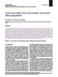
F I G U R E 1 Principal component analysis performed at the individual level. European individuals were plotted using blue dots, whereas American individuals were plotted with red and green dots. Green dots represented American individuals located within the European dot cloud beyond the limit of the ellipse related to American individuals. Ellipses were plotted to illustrate the identified genetic clusters. They encompassed roughly 95% of the individuals of each range
interpolation using individual membership coefficients for the most likely K within each range. An inverse distance weighting (IDW) in‐
and (c) within populations and were as follows: observed heterozygos‐
terpolation with a power value of 1 was carried out using the ArcGIS
ity (Ho), which quantifies the proportion of heterozygous individuals;
v10.2.2 geostatistical analyst tool (ESRI, 2011). The neighborhood
expected heterozygosity (He), also known as genetic diversity, that
was searched using a four sectors circle with a maximal value of 25
measures the expected proportion of heterozygous individuals under
neighbors and a minimum of 0.
Hardy–Weinberg Equilibrium; allelic richness (AR), which corresponds to the number of alleles weighted by the number of individuals in the
2.3.3 | Analysis of genetic differentiation and diversity
smallest population; inbreeding coefficient FIS within each population that measures the proportional deviation of observed from expected heterozygosity within subpopulation; and the total number of alleles
The genetic differentiation between populations (with values be‐
(TNA) per range, calculated by summing within each range the number
tween 0 and 1, none‐full differentiation) was analyzed using FST
of allele over all loci.
indexes (Wright, 1931). Within and between ranges, FST were cal‐
Differences in AR were determined by performing a nonpara‐
culated with the hierfstat v 0.04‐28 R package (Goudet, 2005) ac‐
metric Wilcoxon paired test among loci between ranges. In order
cording to the Weir and Cockerham method (1984). 95% confidence
to evaluate differences in total number of alleles between ranges,
intervals (CI) were estimated by performing 1,000 bootstraps over
a bootstrap over all loci and individuals was computed using 1,000
loci.
simulations and the differences were determined using a nonpara‐
Two datasets were analyzed in order to compare genetic diver‐ sity between ranges: the initial dataset (818 individuals minus 98
metric Mann–Whitney test using R version 3.3.1 (R Development Core Team, 2016).
clones = 720 genotyped individuals using 113 SNPs) and the additional dataset (163 genotyped individuals using 251 SNPs, see Section 2). The second dataset specifically aimed to test for a potential bias in allelic
2.3.4 | Isolation by distance analysis
frequency due to SNP selection. First, allelic frequencies were evalu‐
In natural populations, genetic similarity is expected to be high
ated by plotting the MAF (Minor Allelic Frequency) distributions per
between spatially close populations and then to decrease among
locus and per range. Using the R package Hierfstat v 0.04‐28 (Goudet,
populations with geographic distance; this pattern is known as iso‐
2005) and Fstat software v2.9.3 (Goudet, 2013), diversity indices were
lation by distance (IBD). IBD was tested within each range, using
calculated (a) between ranges, (b) among populations within ranges,
two approaches: (a) The genetic distances between populations
|
BOUTEILLER et al.
8
F I G U R E 2 (a) Individual assignation for the most likely number of clusters (where K = 2) as a result of the between range STRUCTURE analysis. Each colored vertical line represents one individual ancestry membership between the two clusters (orange, cluster K2_1, and blue cluster K2_2). Black vertical lines separate different populations. Both analyses were computed on the initial dataset after clone removal (720 individuals from 63 populations genotyped using 113 SNPs). (b and c) Pie charts of the population assignation in Europe and the USA for the most likely number of clusters (where K = 2) as a result of the STRUCTURE analysis between ranges. In blue, proportion of individuals significantly assigned to cluster K2_1; in orange, proportion of individuals significantly assigned to cluster K2_2; and in Purple, proportion of individuals admixed in each population. The native distribution of black locust within America (Little, 1971) is plotted in gray shading and in Europe it is present almost everywhere from Southern to Northern Europe were calculated as the ratio FST/(1−FST ) using pairwise FST plotted
TA B L E 2 Isolation by distance correlation tests
against the logarithm of the pairwise geographic distances among
Pearson test
populations (Rousset, 1997) and the correlation was tested using a Pearson coefficient test; and (b) A Mantel test between the matri‐ ces of pairwise geographic distances and pairwise genetic distances was performed using the R ade4 library, with 9,999 permutations of matrices. For both methods, pairwise geographic distances among populations were calculated with the GPS coordinates of each popu‐ lation using the R CalcDists function provided by Scott Chamberlain on GitHub (https://gist.github.com/sckott/931445). The matrix of pairwise genetic distances was estimated using the Cavalli‐Sforza and Edwards Chord distance with hierfstat v 0.04‐28 (Takezaki & Nei, 1996).
Range USA
r 0.53
Mantel test
p 2.9 × 10
r −30
0.193
1.28 × 10
Ozarks
0.386
0.27
Europe
r
0.75
K2_1:
0.105
0.223
K2_2:
0.0692
0.483
Appalachians
p 0.479
3 × 10 −4
−3
−0.028
0.562
Note. Both regression of pairwise FST/(1 − FST ) on logarithm of pairwise geographic distance (Rousset, 1997) and a Mantel test were performed within each range or within a subselection of the population in each range. Significant results are in bold.
3 | R E S U LT S 3.1 | More asexual reproduction in European populations
(χ 2 = 29.04, df = 1, p = 7.10 × 10⁻⁸). As expected, no clone was found within the common garden populations, nor in the populations ob‐ tained from seedlings germinated in the laboratory. When removing
Overall, a higher clonality was detected in the European popula‐
these populations from the analysis (thus leaving 280 European and
tions compared to the American ones, with a significant range effect
356 American individuals), 98 genotypes were found with a least one
|
9
BOUTEILLER et al.
F I G U R E 3 (a and b) The graphical IDW interpolation computed on the STRUCTURE for individual ancestry membership for each within range analysis. Results are shown for the most likely K in Europe and in the USA, K = 2 and K = 3, respectively. IDW within America is plotted over native distribution of black locust. The two European clusters are represented by a continuous color scale from blue (K2_1_EU) to red (K2_2_Eu). The three clusters in the USA are represented by a continuous red color scale (K3_1_US) through to a blue color scale (K3_2_US) and green color scale (K3_3_US)
duplicated version (i.e., clones): 68 clones out of the 280 European
the northeastern part of its native range. Among the 29 sampled
samples and 30 clones out of the 356 American samples. Keeping
American populations, only four (Altoona, Eriline, US Grp 3, and
only one sample per genotype resulted in a dataset that contained
Wayne National Forest) showed individuals with a high level of ge‐
720 genotypes out of the 818 sampled individuals after clone re‐
netic relatedness to the European individuals. The structure and
moval, which was distributed as 334 genotypes in 34 European pop‐
multivariate analyses gave congruent results.
ulations and 386 genotypes in 29 American populations.
First we used a PCA (Figure 1) to analyze the position of individu‐
Among European populations (Table 1), the index of clonal diver‐
als on the factorial plan. Axis 1 roughly separated European (in blue)
sity R ranged from 0.27 to 1 (mean = 0.82, SD = 0.26), with significant
and American (in red and green) individuals in two partially overlap‐
differences in clonality between populations (χ 2 = 88.33, df = 60,
ping clusters. A few American individuals (in green) were present in‐