With an increasing requirement for network monitoring ... monitoring of network flows. However .... router vendors such as Cisco and Juniper to support a simple.
A Framework for Efficient Class-based Sampling Mohit Saxena Ramana Rao Kompella CSD TR #08-022 September 2008
A Framework for Efficient Class-based Sampling Mohit Saxena and Ramana Rao Kompella Department of Computer Science Purdue University West Lafayette, IN, 47907 Email: {msaxena,kompella}@cs.purdue.edu
I. A BSTRACT With an increasing requirement for network monitoring tools to classify traffic and track security threats, newer and efficient ways are needed for collecting traffic statistics and monitoring of network flows. However, traditional solutions based on random packet sampling based treat all flows as equal and therefore, do not provide the flexibility required for these applications. For example, network operators are often interested in observing as many unique flows as possible; however, random packet sampling is inherently biased towards large flows thus making it unsuitable for such application. Operators may also be interested in increasing the fidelity of flow measurements for a certain class of flows, which cannot be achieved in such frameworks. In this paper, we propose a novel architecture called CLAMP that provides an efficient framework to implement class-based sampling. At the heart of CLAMP is a novel data structure called Composite Bloom filter (CBF) that consists of a set of Bloom filters that work together to encapsulate various class definitions. We show the flexibility and efficacy of CLAMP by implementing two-class size-based sampling. We also consider different objectives such as maximizing flow coverage and improving the accuracy of certain class of flows. In comparison to previous approaches that implement simple size-based sampling, our architecture requires substantially lower memory (upto 80x) and results in higher flow coverage (upto 8x more flows) under specific configurations. II. I NTRODUCTION Flow monitoring is an essential ingredient of network management. Typical flow monitoring involves collection of flow records at various intermediate network boxes such as routers. These flow records can assist a network operator in various tasks such as billing and accounting, network capacity planning, traffic matrix estimation, and detecting the presence of adversarial traffic (e.g., worms, DoS attacks). While the basic task of flow monitoring appears simple, collecting flow records at high speeds under extremely resourceconstrained environments is quite challenging. Particularly, memory and CPU resources in routers are often distributed among several critical functions such as route computation, forwarding, scheduling, protocol processing and so on, with the result that flow monitoring tasks receive only a small fraction in the overall pie. With such constrained resources and ever increasing link speeds, it is extremely difficult to
record each and every packet on a given interface. In order to overcome this hurdle, routers record only a random subset of packets that they observe by sampling the packets that traverse the interface. The rate at which packets are sampled typically depends on the resources available on the router. The three major router resources that the task of flow collection task needs to grapple with includes CPU, memory, and flow export bandwidth. Several sampling schemes exist to control the utilization of these resources. For example, Cisco’s flow collection tool called NetFlow [4] implemented on routers includes a simple stage of random packet sampling. These schemes export flow records computed on an unbiased sample of packets collected on each interface. These unbiased flow records could then be used to estimate flow aggregate volumes. For example, these flow records could be used to estimate the volumes of popular applications such as Web and Email, or volume of traffic going from one prefix to another prefix for traffic matrix estimation. One major deficiency of uniform packet sampling in collecting flow records is its bias towards heavy-hitter flows, i.e., flows that have a large number of packets. Given that Internet flow size distribution is heavy-tailed, a large majority of sampled packets typically belong to a few large flows. While such a bias does not affect volume estimation applications, it provides no flexibility to network operators to specify how to allocate their overall sampling budget among different classes of traffic. For example, an operator might want to specify that he is interested in collecting as many small-sized flows as possible to satisfy security applications such as tracking botnets, detecting portscans and so on. For such applications, packet sampling is exactly the wrong choice as it inherently fills up the sampling budget with a large number of packets from “elephant” flows. In general, we observe that while sampling budget is directly dictated by router constraints, the network operator should be able to specify how to use this sampling budget efficiently to satisfy monitoring objectives. The monitoring objectives themselves are context and location dependent, and as such, a flexible architecture is desired which can accomodate several ways of allocating the sampling budget among different types of flows. It is, however, not feasible to control the sampling on a per-flow basis due to two reasons. First, the number of flows is too large which means a lot of state needs to be maintained. Second, it causes tremendous administrative overhead to configure and manage the sampling rate.
2
Instead of fixing a per-flow sampling rate, it is beneficial to aggregate flows into classes and allocate specific sampling rates to these individual classes. Note that this is similar to how we achieve QoS in modern routers through aggregation into DiffServ classes. Indeed, newer versions of Cisco’s NetFlow [3] allows setting input filters which allow specifying different filters for different classes of traffic. However, the definition of a class is based on an access control list and thus is based primarily on the fields of the header. We cannot, for example, specify that small flows and large flows get different sampling rates to implement size-based sampling [9]—a serious limitation of this static class-based sampling. In this paper, we propose an architecture, called CLAMP, that provides network operators to define dynamic flow classes (i.e., those that are not dependent only on static header fields) and perform efficient class-based sampling on these flow classes. While the architecture of CLAMP is generic, and can potentially support several newer and more flexible varieties of sampling, we focus on implementing simple two-class sizebased sampling in this architecture as a canonical example to illustrate the efficacy of our approach. While allocating different sampling rates to different types of flows based on their flow sizes has been proposed before in [9], the simplicity of our architecture facilitates an implementation with significantly less memory and high accuracy. Thus, the contributions of our paper are as follows: • We describe the architecture of CLAMP that achieves dynamic class-based sampling with the help of a novel classification data structure called Composite Bloom Filter to help network operators flexibly allocate different sampling budgets among different competing classes. • We show how to perform simple two class size-based sampling (with extension to multiple classes) using our architecture. We also consider how to specify different objectives such as increasing flow coverage and maximizing accuracy of a specific group of flows and so on. • We present both theoretical as well as empirical analysis for the same. Our results using real traces indicates that our architecture consumes up to 80x less memory and results in larger flow coverage (upto 8x more flows under specific configurations), as compared to existing solutions. The rest of the paper is organized as follows. First, we provide background and related work in Section III. We then describe our the CLAMP architecture in Section IV and implementation details of size-based sampling in Section V. We outline evaluation details in Section VI. III. BACKGROUND AND RELATED WORK The increasing importance of flow measurement as an essential ingredient in several network management tasks prompted router vendors such as Cisco and Juniper to support a simple flow measurement solution called NetFlow [4] in routers. The basic version of NetFlow observes each and every packet on a given router interface and checks to see if a flow record is already created for that given packet. If it is already created,
the information from the packet is incorporated into the flow record. The basic form of NetFlow maintains simple flow statistics such as packet and byte counters and information about TCP flags, timestamps of the first and last packet among other information. Thus, on each packet, the flow record corresponding to the packet is found and the packet counter and byte counters are incremented while also noting if there are any special flags in the packet. Basic NetFlow does not scale beyond a few flows and at high link speeds and thus is not suitable for several core backbone links. Routers, therefore, support sampled NetFlow, a variant of NetFlow that works on packets that are sampled according to a configurable sampling rate (say 1 in 64). By randomly sampling packets, sampled NetFlow allows unbiased estimators to compute volume estimates for different types of traffic. Several flow monitoring solution that exist in the literature are fundamentally based on this simple idea. For example, adaptive NetFlow [5] adapts the sampling rate in the presence of adversarial traffic mixes to control resource usage. FlowSlices [8] advocates the use of different tuning knobs for different resources (memory, CPU and reporting bandwidth). ProgME [12] provides a way to specify which flows a network operator is interested in based on constructing binary decision diagrams that can in turn be programmed into the router. While random sampling is easy to implement, it is not necessary the most effective form of sampling depending on what is desired. For example, the inherent bias of random packet sampling towards large flows might be harmful if collecting as many flows as possible is the objective. More generally, they either do not distinguish between different classes of traffic (e.g., adaptive NetFlow and FlowSlices) or they explicitly pick the flows (using packet headers) they want to monitor and do not sample sub-populations within a category (e.g., ProgME). A seminal paper by Kumar et. al [9], addresses this limitation and provides a way to perform size-dependent sampling using a sketch to estimate the flow size. By configuring the sampling rate to be inverse of the flow size, the relative error of flows irrespective of the flow sizes remains similar. Note that this is unlike random packet sampling in which flow size estimates for large flows exhibit much better accuracy as compared to smaller flows. Their main observation is that we can reduce the sampling rate for large flows and allocate more sampling budget towards smaller flows so that the accuracy of large flows only decreases by a little while small flows benefit significantly. Given they need flow size estimates, they advocate the use of an online sketch to obtain flow size estimates. FlexSample [11] builds upon this basic idea and attempts to explicitly improve the flow coverage, as opposed to just accuracy of volume estimates. Both these solutions, however, use sketches or counting Bloom filters which are quite heavyweight. In addition, they are too atuned towards size-dependent sampling and do not provide explicit ways to specify how to maximize the flow coverage or accuracy of a particular group of flows. Our architecture, on the other hand, is much
3
1 0 1 0
Packet Stream
Composite Bloom Filter
[1]
[1]
[0]
Class Membership Bit Map [1101]
[1]
Sampling Process Sampling Rate = f([1101]) Sampled Packets
Packet Classifier
Feedback: Insert Action
Flow Memory
Flow Records
Fig. 1.
Architecture of CLAMP.
more generic and also uses light-weight data structures for classification thus reducing the overall memory consumption as well as improving the flow coverage or accuracy depending on the specific objective, as we discuss next. IV. D ESIGN
OF
CLAMP
Our goal is to design an architecture that provides flexibility in configuring different sampling rates for different types of flows. Thus, the design of CLAMP comprises of two basic components—a classification data structure called Composite Bloom Filter (CBF) and flow memory as shown in Figure 1. Each packet upon its arrival is passed through the CBF to first identify the class to which the packet belongs to. CBF is composed of a few Bloom filters (BFs) working in tandem to provide hints about the class to which an incoming packet belongs to. Since the CBF uses simple BFs, it is small enough to fit well in fast memory (SRAM) and can easily operate at link speeds such as OC-192 and OC-768. Generally speaking, a specific combination of BFs represents a class. Thus, upon each packet arrival, the packet’s flow id (e.g., the 5-tuple) is queried parallelly within each BF and the matching BF indices are obtained. The tuple of matching BFs is used to identify the class to which the packet belongs to. In the simplest case, each BF represents a unique class; thus, the number of classes equals number of BFs and the packet that matches a given BF is said to belong to the corresponding class. In more complex scenarios, class definitions include arbitrary combinations of BFs. As shown in Figure 1, the sampling rate corresponding to each packet is determined by first identifying the class to which the packet belongs to. The network operators can choose the sampling rate for a class based on several criterion. For example, network operators may want to sample a given target fraction of packets for different classes subject to processing constraints. They may also want to increase the accuracy of volume estimates for certain types of flows. In addition, they can also choose to allocate flow and packet coverage over different flow classes in a ‘fair’ manner. We discuss a few such objectives in more detail in Section V-B. Once the sampling rate is determined, the packet is then probabilistically sampled based on this rate. If the packet is sampled and a flow record exists in the flow memory, then the flow record is updated with the contents of the packet (e.g.,
packet counter is incremented, byte counter is incremented by the packet size, and special flags in the packet are noted). If not, a new flow record is created for this packet. We envision that the flow memory resides in the larger and less expensive memory (DRAM)1 . Flow memory is periodically reset when the flow records are reported to the collection center. The most important step is to decide which flows are inserted into a given BF. If classes are just based on pure packet headers, it is relatively straightforward to insert individual flows into the BFs. However, classes can be dependent on specific flow characteristics such as packet or byte counts. Such flow characteristics are not known a priori and must be determined on-the-fly. Even further, a flow may initially belong to a class X and then may transition into class Y at a later time. In order to account for such dynamics, we use the flow records in the flow memory to determine which class a given flow belongs, and when a flow transitions from one class to another. This is depicted as the feedback action in Figure 1. Note that BFs do not allow deletion of flow records; thus, once a flow is entered in a given BF, it cannot be deleted from that BF. This may constrain the flow definitions to some extent. Because records in the flow memory are based on sampled packets, they are subject to renormalization errors. When flows are inserted or transitioned between different classes based on these sampled statistics, these renormalization errors can effect the accuracy of the mapping between a flow and a class and thus may result in misclassification of certain flows. In addition, there could be misclassification due to the inherent false positives associated with BFs. To some extent, this is unavoidable due to the approximate nature of the data structure; the key is to ensure that such misclassification results do not significantly affect the overall flow monitoring objectives. While the framework itself is quite general, we focus on one specific example, namely size-based sampling, to illustrate the efficacy of CLAMP. V. S IZE - BASED SAMPLING
USING
CLAMP
It is well known that sampling random packets for collecting flow statistics is prone to biases towards larger flows [9]. To alleviate this problem, an operator may like to, for example, set different sampling rates for ‘mouse’ and ‘elephant’ flows, where a flow is termed a mouse or an elephant depending on whether the number of packets in that flow is below or above a particular pre-defined threshold, T . By setting a higher sampling rate to mouse flows, we will be able to capture a larger number of unique flows, or in other words, increase flow coverage. This however, may result in a reduction of the accuracy of flow volume estimates for the elephant flows. Both of these might be perfectly valid objectives for a network operator; the choice of one over the other depends on the particular scenario. We consider both of these choices. 1 In some cases, a limited amount of flow memory may reside in SRAM which is then flushed to the DRAM
4
T2
k hash fns
>
T1
Virtual filter
Flow Label E2
E1
M
Packet
Search order Composite Bloom Filter
Fig. 2.
CBF: Finding the flow class to which a packet belongs.
A. Configuring the CBF In this section, we discuss how we can configure the CBF to implement different sampling rates for both the mouse and elephant classes. In this case, the CBF comprises of two Bloom filters naively, one for the mouse and the other for the elephant flows. However, since every flow starts off as a mouse flow as we do not know the flow size a priori, there is no explicit need for a mouse Bloom filter in the CBF. The two basic operations on CBF are find and insert. For each packet, the five tuple corresponding to the source and destination IP addresses and ports along with the protocol field is used to uniquely identify a flow. As shown in Figure 2, this flow five-tuple is hashed using k hash functions in parallel, and the hashes are queried in each of the k Bloom Filters in parallel. The matched class with the highest priority is picked. In our case, if a flow belongs to the elephant class, then both the elephant and mouse BFs (if existed) will respond with a match, and since the priority of the elephant class is higher, the flow belongs to that class. More generally, all the BFs are arranged in priority of increasing flow sizes Figure 2 shows the case with three BFs for three classes—E2 , E1 and M . E2 and E1 classes are distinguished with the threshold T2 and E1 and M by T1 . Since T2 is greater than T1 , E2 has higher priority than E1 , which in turn has higher priority than M . Initially, all flows are entered in the mouse filter upon the arrival of the first packet. A new entry is created for a flow in the elephant filter, if the flow crosses the threshold to become an elephant. This particular operation can be seen as the feedback from the flow memory to the CBF in Figure 1. Flow memory, however, is updated for every packet sampled for a flow. B. Analysis For our example of a two-class CBF, packets can be classified into either mouse or elephant packets, with some mouse packets misclassified as elephant packets and viceversa. We use MM and ME to denote sampled mouse packets that are classified as mouse and elephant packets respectively (and hence sampled at mouse and elephant sampling rates). Similarly, we denote EM and EE as the elephant packets classified as mouse and elephant packets respectively.
If we used exact flow counters, ME would be zero, since a mouse packet would never be misconstrued as an elephant packet. However, due to the inherent false positives associated with BFs, there might be an occasional match of a mouse flow within the elephant BF causing ME to be non-zero. The probability of such collisions is β = (1 − ekn/m )k , where k is the number of hash functions, n is the number of elements supported by the filter, and m is the size of the filter [7]. On the other hand, EM exists because of the inherent online nature of our framework; a flow is deemed mouse until enough packets arrive to qualify for an elephant, thus initial packets are always misconstrued as mouse. For any sampling framework, the most fundamental constraint is applied by the processing limits. We define c as the capacity or the maximum number of packets which can be sampled at a given rate constrained by the processing power. More formally this basic resource constraint inequality can be written as follows: N = MS + ES ≤ c where N is the total number of packets sampled and MS and ES are the actual number of packets sampled which belong to mouse and elephant flows respectively assuming an oracle which can perform perfect classification. From our definitions, MS = MM + ME and ES = EE + EM . Due to misclassification of mouse packets as elephant, some of the mouse packets are sampled at elephant rate. Hence, we need to reduce this fraction from MM and add it to ME . Thus, we get the following: MM = sM · M · (1 − β) M E = sE · M · β
(1)
where, sM and sE are the sampling rates of the mouse and elephant classes and M is the total number of mouse packets. Generally, at larger sizes for the filters, β will be small enough to approximate MM to be simply equal to sM ·M . Similarly, every elephant flow in the beginning of its evolution is treated as a mouse flow, until an estimated T /sM packets have been encountered for it, where T is the threshold number of sampled packets at which a flow changes from mouse to elephant. EM ≤ FE · T EE = sE · (E − EM /sM )
(2)
where FE is the total number of elephant flows and E is the total number of elephant packets. Note that EM is atmost FE times the threshold T , since a flow will be immediately labeled as an elephant once T packets are sampled for that flow. Hence, we need to reduce these many packets sampled at mouse sampling rate, to get the expression of EE . We now plug in the values for MM , ME and EE to derive a more general inequality (assuming negligible values for β), as follows: N ≤ sM · M + FE · T + sE · (E − EM /sM ) ≤ c
(3)
5
Using this general inequality, we will now show how a network operator can compute appropriate values for sM and sE to configure a general two-class size-based sampling, to satisfy the resource constraints and at the same time maximize his metric of interest—flow coverage or accuracy or both. Maximizing flow coverage: One of the main objectives we consider is increasing the number of unique flows captured by CLAMP, either for a particular group or for all the flows. Due to the heavy-tailed nature of Internet traffic, there are many mouse flows with a few elephants. To increase the flow coverage of mouse flows, we need to increase the sampling rate sM . However, for a given sampling budget and processing constraints, we cannot increase it indefinitely. The Equation 3 is a quadratic in sM that can be solved to obtain the following solution for sM . p sM = (t + t2 + 4sE · EM · M )/(2 · M ) (4) where, t = c − sE · E − EM All positive values of sM less than the one defined above will satisfy the processing capacity c. We can get estimates for E, M and EM historically, based on the past measurement cycle(s). Due to the heavy-tailed nature of Internet traffic, maximizing the value of sM will automatically lead to increasing the overall flow coverage. Thus, we maximize the value of sM with respect to sE to obtain the values for sM and sE that will lead to maximizing the flow coverage. sM = min{(c − EM )/M, 1} sE = max{0, (c − M − EM )/(E − EM )}
(5)
In most cases, the first configuration with sM set to (c − EM )/M and sE to 0 would work fine because sampling capacity c is typically very small. Only when we have higher sampling capacity, we will need to configure sM to 1 and sE to a value less than or equal to (c − M − EM )/(E − EM ), so as not to underutilize the spare sampling capacity. We refer to this sampling scheme as sample and block as it is the opposite of sample and hold [6] that is designed to identify large flows. Sample and block samples packets belonging to mouse flows at the maximum possible sampling rate sM , and as soon as a mouse flow becomes an elephant, it stops sampling further packets for that flow. Thus, it tries to allocate most of the sampling budget for identifying the mouse flows. It is useful to compare the coverage gains of such an approach with that of random packet sampling with probability sR . To perform fair comparisons, the invariant we maintain is the sampling budget c in both schemes. We compute the maximum packet coverage gain for mouse flows obtained at this configuration, as follows: (c − EM )/M c/(M + E) = (1 + E/M ) · (1 − EM /c) for EM < c ≤ (M + EM )
Gmax = (sM · M )/(sR · M ) =
(6)
While Gmax is actually packet coverage gain, it is directly related to the flow coverage gain for mouse flows, because all the mouse flows have less than or equal to T packets. We note that Gmax is dependent on two terms: 1+E/M and 1−EM /c. The first term is solely dependent on the traffic mix or the trace characteristics. However, the second term is dependent on the amount of misclassification occuring for elephant flows. Note that the gains in mouse coverage Gmax are due to the reduction in number of elephant packets sampled and increase in the sampled mouse packets; the sum of both these sampled packets is the same as that of random packet sampling. Along with increasing the packet and flow coverages, sample and block can also increase the accuracy of the flow size estimates for the mouse flows, as we discuss next. Maximizing accuracy: CLAMP when configured to sample and block, achieves the maximum packet and flow coverage for mouse flows. Because mouse flows consist of only a few packets, an increase in their coverage directly results in increased accuracy for their volume estimates. However while maximizing for flow coverage, we tradeoff with the accuracy of medium and large flows. In order to improve their accuracy or reduce their relative estimation error, we need to shift the equilibrium of our sampling budget towards them. Earlier work has shown that random packet sampling is biased towards sampling these heavy-hitters and achieves sufficiently good accuracy for their flow size estimates. In order to achieve accuracy atleast as good as random packet sampling, we must sample atleast those many elephant packets. This can be simply achieved by configuring both sM and sE equal to sR . As we reduce sM from its value for maximum coverage, and increase sE to compensate for the reduction in N , accuracy in flow size estimates for medium and large flows increase. Thus, the network operator has the flexibility to configure CLAMP for achieving maximal flow coverage for mouse flows, along with sufficiently accurate flow size estimates for medium and large flows. This can be attained by tuning to a point between the configurations for maximum coverage and maximum accuracy. Further, this analysis can be easily extended to multiple classes by computing the sampling rates corresponding to each class one at a time, based on the requirements of the network operator. VI. E VALUATION While we envision CLAMP to be implemented in hardware for high speeds, we built a prototype software implementation of CLAMP for evaluation. This prototype required nearly 1200 lines of C++ code. The most important component of CLAMP is the packet classification data structure, which is implemented as a vector of binary Bloom filters (hash tables). Our prototype allows selecting the number of hash functions (k), number of entries (m) in each filter and even the epoch size (e). We use Bob Hash function as suggested by [10] for packet sampling at line speeds. Each hash function is initialized with a different 32 bit value.
6
Name ABIL CHIC
Date/Time 2002-08-14/09:20 2008-04-30/13:10
Duration 600s 60s
Online Source www.nlanr.net www.caida.org
Link OC-48 OC-192
Mbps (Kpkt/s) 294.2 (57.6) 971.4 (217.4)
Packets 34,573,317 13,046,322
5-tuple flows 2,195,366 1,174,965
TABLE I T RACES USED FOR OUR MEASUREMENTS .
False positive rate β vs. memory usage 1
0.8
0.8
False positive rate
Fraction
Mouse flow coverage vs. memory usage 1
0.6 CBF Counting BF
0.4 0.2 0
0.6 CBF Counting BF
0.4 0.2 0
1
2
3
4 5 6 7 m/n ratio: Memory usage
8
9
10
(a) Flow coverage Fig. 3.
1
2
3
4 5 6 7 m/n ratio: Memory usage
8
9
10
(b) False positive rate
Effect of varying memory usage for CBF and counting BF (T=1,sM =1,epoch=600s).
Using this prototype implementation, we evaluate the efficacy of CLAMP over real-world traces. We also implemented other size-based sampling frameworks [9], [11] and use these in our comparisons. We show how to configure CLAMP to obtain better flow coverage using our theoretical analysis in Section V-B. We also discuss how CLAMP can be configured for maximizing the mouse flow coverage and accuracy by employing the sample and block scheme. Finally, we show the results on accuracy of flow size estimates by CLAMP, for large flows and compare them with random packet sampling. We used two real-world anonymized traces to analyze the performance of CLAMP. The first is a 10 minute OC-48 trace published by NLANR [2] with 34 million packets and about 2.2 million flows, while the second is a 1 minute OC-192 backbone trace of a tier-one ISP published by CAIDA [1] with 12 million packets and 1.1 million flows. Both traces exhibit heavy-tailed flow size distributions that we assume in our analysis. These traces are summarized in Table I. A. Memory Usage In this section, we compare CLAMP with other counterbased schemes for size-based sampling such as FlexSample [11] and sketch-guided sampling [9]. While the focus and usage of these solutions is different, they both share similar data structures (sketch and counting Bloom filters) to keep track of the flow sizes. In contrast, we rely on CBF that represents a much simpler data structure. In many cases, such simplicity comes at the cost of worsening some other metric such as, say, increasing the false positive rate of the filter. The results indicate, somewhat surprisingly, that CBF performs better in both memory consumption as well as false positives compared to counting BF alternatives, thus indicating that CBF achieves clear benefit and is not a tradeoff.
Why is higher false positive rate in the classification data structure bad for various sampling objectives ? As an example, consider the case when we are interested in increasing flow coverage. According to Equation 1, the mouse flow coverage is directly related to the number of mouse packets classified and sampled at mouse rate MM . Mouse flow coverage, however, decreases as filter false positive rate β increases as these packets will be mis-classified as elephant packets and thereby sampled at elephant rate (i.e., less than the mouse rate for high flow coverage). Thus, low false positive rate for the classification data structure is important for such objectives. In Figure 3(a), we compare the mouse flow coverage (which is equal to MM for T set to 1) for the full ABIL trace for CLAMP and counting BF. In addition to the mouse flow coverage, we also plot the empirical values for filter false positive rate β (calculated using Equation 1) in Figure 3(b). The configuration allowed mouse flow coverage to be maximum, i.e., sM set to 1, thus ensuring a worst case analysis for the filter with the maximum number of flows inserted in the Bloom filter over the trace. To ensure fair comparison, we use three hash functions for both CBF as well as the counting Bloom filter. Figures 3(a) and 3(b) show that CLAMP as well as counting BF implementations exhibit a reduction in the false positives and increase in the flow coverage as we increase the amount of over-provisioning (m/n). However, clearly, CLAMP exhibits much faster increase in mouse coverage and decrease in false positives (or misclassifications). CBF achieves a filter false positive rate of 6% at a m/n ratio of 4 (using 174.5KBytes of memory), giving nearly 94.3% mouse flow coverage (at sM =1 and sR =0.069). Note that we do not have 100% mouse flow coverage due to the fact that ME is not zero. At the
7
Epoch size 5s 10s 20s 40s 60s
sR 0.208 0.179 0.157 0.147 0.134
EM 2,141,542 1,757,734 1,477,898 1,344,678 1,179,340
EM /c 0.789 0.754 0.720 0.701 0.676
TABLE II E FFECT OF VARYING EPOCH SIZE (CHIC TRACE , T=1).
same sampling rate, the counting Bloom filter implementation required a m/n ratio of 10 (using 13,960 KBytes of memory) to achieve the same filter false positive rate of 6%. This shows that CBF requires nearly 80x less high-speed SRAM than a counting Bloom filter to achieve similar filter false positive rates and flow coverages. On the other hand, even considering only same number of entries (bits and counters) across both CBF and counting Bloom filter, CBF still obtains at least up to 6x reduction in the number of false positives (at m/n = 5, CLAMP has about 4% false positives while counting Bloom filter experiences about 25% false positives). What makes these gains even more significant is the fact that we do not consider the extra overhead associated with counters (in the counting Bloom filters). If we factor in this disparity, the benefit associated with CBF will increase even further. B. Effect of varying epoch size We show the breakup of EM and sR corresponding to achieving maximum mouse sampling rate (i.e., sM = 1) and for different epoch sizes in Table II. Note that we have overprovisioned the memory for CBF to 436.25 KBytes (m/n = 10) for all epoch sizes to completely eliminate the affects of filter false positives. We reset both the flow memory and CBF after every epoch. We note that for each of the configurations in Table II, packet and flow coverage for mouse flows is very close to 100% (not shown in the Table). From the table, we can observe clearly that as we increase the epoch size, the effective contribution of EM to the total sampling budget reduces. Still, the contribution of EM to c at an epoch of size 60s is still significantly high (EM /c ∼ 0.676) which results in a higher equivalent sR (to obtain a mouse coverage of 1). We note that this problem is inherent in any size-based sampling framework which is used for an online traffic analysis without the prior knowledge of elephant flows. However, a simple optimization to our CBF, namely not resetting the CBF in every epoch, can solve it to some extent, as we see next. C. Effect of resetting the CBF Resetting the flow memory after every epoch is required to meet the constraints imposed by the memory (DRAM) of the sampling device. On the other hand, resetting CBF is useful especially if the amount of memory allocated to CBF is small. Otherwise, the Bloom filters will be filled up too fast rendering it almost useless for classification. Resetting the CBF frequently may result, however, in a considerable increase
in EM . Thus, while resetting both CBF and flow memory is important, a critical question is whether to reset one or both or none of these every epoch. In Table III, we consider three strategies—all reset every epoch, flow memory reset every epoch (of 10s) but no CBF reset for this trace (of duration 60s), and no reset. In each of these strategies, our aim is to achieve the best possible flow coverage; thus, we configure CLAMP with sM equal to 1 and the epoch size is 10s (OC-192 trace). We observe that only flow memory reset case is almost as good as no reset, in terms of EM and mouse packet coverage MM , but with slight increase in total number of sampled packets (can be seen from the calculated sR to achieve the same level of coverage). But resetting the CBF too frequently (as in the all reset case) leads to a much larger number of EM packets unnecessarily, thereby reducing the sampled mouse packets. D. Flow coverage According to Equation 5 and Equation 6, the best possible coverage for mouse flows can be achieved by setting CLAMP in sample and block mode with T =1. Table IV shows the results for ABIL trace with epoch size of 600s and CBF allocated 436.25 KBytes of memory. We note that the theoretical gains for mouse coverage follow Equation 6. Those gains are formulated for the mouse flows which are all such flows with size less than or equal to T packets (T =1). However, in Table IV we show the gains for flows of size 0-1000 packets, which will be slightly less than those obtained for mouse flows according to Equation 6. The flow coverage gains for the overall traffic volume are also mainly decided by the mouse flow coverage , because large flows are almost always captured. We can observe from Table IV that, as we increase the random sampling probability sR , the coverage gain of CLAMP increases from 3.74x (at sR = 0.001) to almost 8.32x (at sR = 0.073). Further increasing sR will reduce the gain since at sR = 0.073, the mouse sampling rate sM can already be set to 1 and cannot further increase the flow coverage. As mentioned earlier, even with sM = 1, we can see that CLAMP almost captures 99.4% of traffic (with the remaining 0.6% attributed to the false positive probability associated with the elephant Bloom filter). Thus, we can clearly conclude that CLAMP provides an order of magnitude better coverage for this traffic mix as compared to random packet sampling. For the CHIC trace, we show the results in Table V. A maximum gain of 84% is achieved for this trace at a random packet sampling rate of 0.307, while at lower sampling rates (sR =0.016), the gains are just 11%. There are two important observations: First, at very low sampling rates (∼0.001), CLAMP is almost as bad as random packet sampling since there is not enough sampling budget mouse flows can ‘steal’ from elephants to improve their coverage. Second, at high sampling rates such as 0.307, we get a gain of 84% which is not as good as we obtained for the ABIL trace (8.32x at sR =0.073). This is in part because of the flow size distribution of CHIC trace (see Equation 6 for the 1+E/M term). But the
8
Case All reset FM reset only No reset (1 epoch)
sR 0.307 0.249 0.239
Packet Sampling 53.8% 47.4% 46.4%
CLAMP 99.2% 99.9% 99.9%
Gain 1.84x 2.11x 2.15x
N 4,017,451 3,255,337 3,115,285
MM 1,738,217 1,755,813 1,755,048
EM 2,279,234 1,499,524 1,360,237
TABLE III E FFECT OF RESETTING CBF AND FM
sR 0.001 0.004 0.016 0.064 0.073
sM 0.0043 0.0267 0.146 0.845 1.0
ON COVERAGE FOR FLOWS OF SIZE
Packet Sampling # Flows Percentage 6,524 0.3% 22,472 1.0% 73,968 3.4% 233,825 10.7% 261,872 11.9%
0-100 PACKETS (sM =1,T=5, EPOCH =10 S ).
CLAMP # Flows Percentage 24,454 1.1% 114,188 5.2% 456,357 20.8% 1,894,616 86.4% 2,179,399 99.4%
Coverage gain 3.74x 5.08x 6.17x 8.10x 8.32x
TABLE IV C OVERAGE FOR FLOWS OF SIZE 0-1K PACKETS (ABIL TRACE ,T=1, EPOCH =600 S , MEMORY =436.25KB YTES ).
sR 0.001 0.004 0.016 0.064 0.307
sM 0.0010 0.0041 0.0179 0.0965 1.0
Packet Sampling # Flows Percentage 5,003 0.4% 19,079 1.6% 69,623 6.0% 216,170 18.7% 622,214 53.8%
CLAMP # Flows Percentage 4,984 0.4% 19,697 1.7% 76,960 6.7% 293,108 25.3% 1,147,231 99.2%
Coverage gain 0.99x 1.03x 1.11x 1.36x 1.84x
TABLE V C OVERAGE FOR FLOWS OF SIZE 0-100 PACKETS (CHIC TRACE ,T=5, EPOCH =10 S , MEMORY =50KB YTES ).
major reason is attributed to the high EM /c ratios for all of these configurations in Table V, because of smaller epoch size (10s) and higher threshold (T =5), effectively decreasing the coverage gain (see Equation 6 for the 1 − EM /c term). However, operating in sample and block mode for the CHIC trace (with T =1, epoch=60s), a lower sampling rate (sR =0.138) results in a much better coverage gain of 3.05x (with only flow memory reset after every 10s), by reducing the share of EM /c. For brevity, we omit those results for CHIC trace. E. Flow size estimation The second objective we consider is to provide flexibility to improve flow accuracy for certain types of flows. We characterize the accuracy of flow size estimates obtained with CLAMP using the mean relative estimation error metric. We calculate the relative estimation error for each flow, and then average it for small groups of flows on the basis of their sizes. For our analysis, we classify flows into three groups—small (0-1K packets), medium (1K-10K packets) and large flows (greater than 10K packets). Getting good estimates for flow sizes of the small flows is really difficult for random sampling because of high quantization errors involved. Increasing the packet coverage for small flows will require allocating a disproportionately higher budget to the small flows as compared to the larger ones. Thus, we configured CLAMP in the sample and block mode with T =1, single epoch and memory 436.25KBytes. Results are shown in Table VI for flows of size 0-1K packets. For each of the points, we started with a base sampling budget (by fixing
sR ) and allocating all this budget the mouse flows (sM is the computed sampling rate) and ignoring completely the elephant flows. As we can see, at sR = 0.073, we could sample all the mouse flows and thus sM = 1.0. We observe at all sampling rates sR , CLAMP achieves much better accuracy than random packet sampling. Of course this result is expected because instead of sampling all the sR · E elephant packets, our approach results in shifting some of this budget to sampling mouse packets. However, the comparisons at very low sampling rates (sR =0.001) are not very meaningful, because both CLAMP and random packet sampling are affected by huge quantization errors. However, for typical sampling rates (sR =0.016) and high sampling rates (sR =0.073), errors are highly reduced for CLAMP. At sR equal to 0.073, for example, CLAMP gives an error of 7% with a standard deviation of 22%. This is almost 105.43x better than random packet sampling. We also note that till a sampling rate of sR = 0.064, all mean relative estimation errors are due to overestimation of flow size estimates. For sR = 0.073, the mean error for CLAMP of 7% is due to underestimation. This is expected because of a high value of sampling rate used for normalization. We show the results for medium (1K-10K) and large (10Kmore) size flows in Table VII. In the table, we start with the sample and block configuration, i.e., sE = 0 and sM = 1.0 and increase sE and reduce sM correspondingly such that the total number of packets sampled remains the same. By increasing sE , we sample more packets corresponding to elephants and thus increase the accuracy of the flow size
9
sR 0.001 0.004 0.016 0.064 0.073
sM 0.0043 0.0267 0.146 0.845 1.0
Packet Sampling # Flows Error Dev. 6,524 342.64 431.50 22,472 96.87 109.91 73,968 28.82 27.64 233,825 8.37 6.55 261,872 7.38 5.65
# Flows 24,454 114,188 456,357 1,894,616 2,179,399
CLAMP Error 91.30 18.39 3.69 0.07 0.07(u)
Dev. 102.34 16.48 2.69 0.28 0.22
TABLE VI A CCURACY FOR SMALL FLOWS OF SIZE 0-1K PACKETS (ABIL TRACE , SAMPLE &
CLAMP sE sM 0 1.0 0.001 0.982 0.004 0.935 0.016 0.75 0.064 0.148 0.128 0.0004 Packet Sampling
# Flows 3,152 3,156 3,156 3,156 3,156 2,307 3,156
1K-10K Error 0.999 0.102 0.019 0.0074 0.003 0.372 0.0017
Dev. 0.0005 0.729 0.349 0.179 0.084 0.694 0.0756
# Flows 594 597 597 597 597 592 597
10K-more Error 0.999 0.091 0.0024 0.0055 0.0007 0.0008 0.0006
Comparison Error reduction Coverage gain 3.75x 3.74x 5.27x 5.08x 7.81x 6.17x 119.57x 8.10x 105.43x 8.32x
BLOCK ,T=1, MEMORY =436.25KB YTES ).
Dev. 5.515 0.245 0.121 0.059 0.029 0.148 0.0262
Coverage 1K-10K 10K-more 99.9% 99.5% 100% 100% 100% 100% 100% 100% 100% 100% 73.1% 99.2% 100% 100%
TABLE VII A CCURACY FOR MEDIUM AND LARGE FLOWS (ABIL TRACE ,sR =0.073,T=1, MEMORY =436.25KB YTES ).
estimates. For example, at sE = 0.064, the mean relative error of medium flows reduces to 0.3% from about 10.2% at sE = 0.001. At this value of sE , CLAMP performs similar to that of random packet sampling. In almost all the cases, the flow coverage remains at almost 100%. Interestingly, small values of sE does not reduce the overall flow coverage as well, as can be seen under the coverage column in Table VII, except when we increase sE beyond sR . This is because large values of sE lead to reducing the value of sM significantly. Given all flows initially start off being mouse, with small sM several medium flows fail to get even sampled to take advantage of higher sE allocated to such flows. VII. C ONCLUSIONS Flow monitoring solutions in routers have evolved significantly over the years from their modest origins in simple NetFlow-like solutions. While most solutions revolve around better handling router resource constraints such as CPU, memory and flow reporting, there is little research on providing an efficient and flexible class-based sampling architecture, with dynamic class definitions that include specific flow properties such as the size. In this paper, we have discussed the architecture of CLAMP to address this challenge that involves the use of a set of simple Bloom filters for class membership and a feedback from the actual flow memory to record classmembership information about flows. Using this architecture, we have shown how to implement a simple two-class size based packet sampling framework. We have analyzed the architecture for this particular application both theoretically as well as empirically using a prototype software implementation over real ISP traces. Our results clearly indicate the simplicity of our approach over the previous solutions. For example, for some configurations, we achieve over 80x reduction in the amount of memory required
for same rate of packet misclassifications. In addition, we have also shown how we can configure the CLAMP architecture for specific network monitoring objectives such as increasing flow coverage and improving the volume estimates of a specific class of flows (based on size). While we have primarily focused on size-based class definitions, our architecture itself is quite generic and lends itself to a wide variety of applications, some of which we intend to pursue in the future. R EFERENCES [1] CAIDA Anonymized 2008 Internet Trace (equinix-chicago collection). http://www.caida.org/data/passive/passive 2008 dataset.xml. [2] NLANR Abilene-I Internet dataset. http://pma.nlanr.net/Traces/long/ ipls1.html. [3] Cisco Systems. NetFlow Input filters. http://www.cisco.com/en/US/docs/ ios/12 3t/12 3t4/feature/guide/gtnfinpf.html. [4] B. Claise. Cisco Systems NetFlow Services Export Version 9. RFC 3954. [5] C. Estan, K. Keys, D. Moore, and G. Varghese. Building a Better NetFlow. In Proc. of ACM SIGCOMM, 2004. [6] C. Estan and G. Varghese. New Directions in Traffic Measurement and Accounting. In SIGCOMM, 2002. [7] L. Fan, P. Cao, J. Almeida, and A. Z. Broder. Summary cache: a scalable wide-area Web cache sharing protocol. IEEE/ACM Transactions on Networking, 8(3):281–293, 2000. [8] R. Kompella and C. Estan. The Power of Slicing in Internet Flow Measurement. In Proc. of IMC, 2005. [9] A. Kumar and J. J. Xu. Sketch guided sampling - using on-line estimates of flow size for adaptive data collection. In IEEE INFOCOM, 2006. [10] M. Molina, S. Niccolini, and N. Duffield. A comparitive experimental study of hash functions applied to packet sampling. In Technical Report, AT&T. [11] A. Ramachandran, S. Seetharaman, N. Feamster, and V. Vazirani. Building a Better Mousetrap. In Georgia Tech CSS Technical Report GIT-CSS-07-01, 2007. [12] L. Yuan, C.-N. Chuah, and P. Mohapatra. Progme: towards programmable network measurement. SIGCOMM Comput. Commun. Rev., 37(4):97–108, 2007.