operates in every vehicle and serves the purpose of real time monitoring and diagnoses of the ... time is vital to maintain a high degree of reliability and safety. ... to confirm the ultimate diagnosis and make repair/recovery recommendations at ...
A FRAMEWORK FOR INTELLIGENT SENSOR VALIDATION, SENSOR FUSION, AND SUPERVISORY CONTROL OF AUTOMATED VEHICLES IN IVHS
Satnam Alag, Kai Goebel, and Alice Agogino Intelligent Systems Research Group Department of Mechanical Engineering, UC Berkeley
ABSTRACT In this paper, we propose a framework for real time monitoring and diagnosis of automated vehicles in an IVHS. The supervisory control methodology proposed here is concerned with fault detection, fault isolation, and control reconfiguration of the many sensors, actuators and controllers that are used in the control process. This supervisory control architecture operates at two levels of the AVCS: at the regulation and at the coordination level. Supervisory control activities at the regulation layer deal with validation and fusion of the sensory data, and fault diagnosis of the actuators, sensors, and the vehicle itself. Supervisory control activities at the coordination layer deal with detecting potential hazards, recommending the feasibility of potential maneuvers and making recommendations to avert accidents in emergency situations. The supervisory control activities are achieved through five modules, organized in an hierarchical manner. Finally, an overview of the different methods that are being used in building such a supervisory controller are stated. INTRODUCTION In order to perform its basic functions (such as longitudinal control, lateral control, platooning, maneuvering techniques, e.g. lane change, exiting the automated lane), the Intelligent Vehicle Highway System (IVHS) requires a large number of sensors for control at the coordination level, the engine level, and for sensing and communication between the vehicles and the IVHS main controller. For all subsystems to work well and reliably the IVHS system requires high sensor data fidelity. However, most generally, sensor readings are uncertain because internal and external sources add noise to the readings or cause a malfunction of the sensor, altogether. Deterministic relationships between the sensor readings and the system being monitored do not exist. No sensor will deliver accurate information at all times. Consequently, the safety of the IVHS system is affected. It is therefore desirable to find a way to avert the negative effect of the shortcomings of the sensors. An inconsistent sensor reading could be a result of a system or process failure, and it is important to distinguish between these types of failure. It is also important to account for the sources of uncertainty and propagate them to the final diagnosis of the system state. Maintaining a high level of safety is an integral part of the IVHS system since it concerns human lives. For the complex IVHS system to work reliably and safely, it must have capabilities for fault accommodation, i.e. have fault detection, isolation and control reconfiguration, which can respond in short time under adverse conditions. Fault accommodation is an important aspect of intelligent control and a challenging problem which often cannot be solved by conventional approaches. It encompasses a diverse collection of technologies and disciplines such as expert systems, neural networks, fuzzy logic, machine learning, and discrete event systems. The key issue for all of these approaches is finding an effective representation for use in converting raw data to features, reasoning with these features and making recommendations consistent with the uncertainty in the measurements, costs, and risks involved
(1). Fault detection deals with the process of identifying if a fault has occurred. A fault event often impairs or deteriorates the system's ability to perform its specified tasks or mission (2). Fault isolation is the ability to distinguish between specific faults and isolating the component that has failed. For fault isolation, measurement of similarity is an important process and has two parts: first, modeling to represent the faults; and second, comparison (for example by using statistical properties) of modeled with sensed signals. Control reconfiguration is the reaction of the system to the findings of the previous two parts of fault accommodation. Depending on the source of the fault (sensor, actuator or process) different means of reconfiguration will ensure a safe reaction. A fault monitoring system should detect as many true faults as possible, while triggering as few as possible false alarms. In addition, the delay time between a fault occurrence and fault detection should be small. In this paper, we develop a framework for real time monitoring and diagnosis of the automated vehicle in IVHS. We propose a supervisory controller which consists of five modules. Within the automated vehicle control system (AVCS) hierarchy, these five modules can be found on two levels, the regulation layer and the coordination layer. This intermediate supervisory controller combines the advantages of having access to the data of the regulation layer as well as the information from the coordination layer. It operates in every vehicle and serves the purpose of real time monitoring and diagnoses of the components in the vehicle and between the vehicle and its environment (other objects in its neighborhood). It is concerned with predicting incipient failures and recommending suitable corrective actions. The main emphasis of this paper is to present a framework for this supervisory control methodology in the IVHS context outlining some of the potential techniques that could be used for each module and the approach taken by us to build the supervisory controller. METHODOLOGY We begin with explaining the significance of the supervisory controller. Next, we explain the meaning of the controller being divided up into two levels within the AVCS architecture. The different modules which the controller consists of are introduced and tools for each module are enumerated. Supervisory Control Architecture Control of the automated vehicle in the IVHS can be divided into two operations, the first deals with the basic lateral and longitudinal control of the vehicle, while the second operation deals with various supervisory tasks. The supervisory tasks consist of indicating undesired or non permitted process states (3) and to take appropriate actions in order to avoid an accident. Normally, faults in the vehicle on the IVHS will affect its performance and control. A fault can be considered as any non permitted deviation in the characteristic property of the vehicle (like a tire burst), the actuator, the sensors and the controllers. Component failure, energy supply failures, environmental failures, maintenance errors etc. are some of the common sources of failure (4). In IVHS, supervisory controllers are required for two different tasks: first to detect faults in the vehicle and the second to detect faults (or deviations) in the environment around which the vehicle is operating. An example of the latter is the development of unforeseen faults in the vehicles' neighborhood due to sudden change in the expected configurations of the collection of vehicles which could be caused by a failure of either the sensors or incorrect response to a stimulus of the controller in one of the automated lanes. This calls for real time fault tolerant action on part of the supervisory controller. Another extreme case is one in which the tires burst and then the entire dynamics of the vehicle changes. In order to accommodate the changes in the engine controller dynamics, the intermediary controller needs to react to the new situation in real time and to come up with an exigency response to either see the maneuver through to completion or to abort it in a fashion which is consistent with the configurations of all the interacting vehicles in a manner which is feasible, safe and quick in its response. For instance the arrival
of an unexpected obstacle (e.g. debris of a previous accident, or an animal) during normal platooning operations as well as midway during the maneuver needs real time decisions to move the vehicle or vehicles involved into a position which avoids any collision or, if unavoidable, to a configuration which minimizes the total damage involved. The supervisory controller also plays an important part during maneuvers. The elementary maneuvers based on the path planning achieved by the coordination layer as suggested in (5), require the individual vehicle to interact with the environment including the vehicles in neighboring lanes via the longitudinal sensors and communication facilities that it is endowed with. Once the vehicle has completed its protocol and has the sequence of maneuvers implemented which it has to carry out, its interaction with the environment and the requirement that it closely monitors changes in them and reacts to them in real time is vital to maintain a high degree of reliability and safety. The vehicle intending a lane change interacts with the vehicles of the neighboring lanes, which may be either members of a platoon or free agents as shown in Figure 1. Once the sequence of maneuvers of the system is decided, it is imperative to have an intermediary supervisory advisor to monitor the progress of the maneuver such as lane merge, split or lane change and see it through to a satisfactory end.
Fig. 1 : Interactions between vehicle and platoons during maneuvers
Since safety is of prime importance in an IVHS system, it is imperative to first validate and fuse the uncertain readings obtained from the numerous sensors. Therefore, the first task to be carried out by the supervisory controller is to validate the sensor readings and get an estimate for the various parameters to be used in the monitoring and fault diagnosis part. Our experience has shown that real time fault diagnosis for complex systems benefits from a hierarchical information processing structure with selecting faults on one level, focusing in more detail on these candidate faults at a higher level, and finally looking for facts to confirm the ultimate diagnosis and make repair/recovery recommendations at
yet a higher level. The approaches taken include the integration of heuristics and model-based reasoning, procedures for fusing qualitative and quantitative data for developing probability assessments, and explicit reasoning about the time constraints inherent in real-time processing of large amounts of data. We therefore propose a multi-level architecture for real time monitoring and diagnosis of the automated vehicle, which consists of the modules for sensor validation, sensor fusion, fault diagnosis, hazard analysis, and a safety decision advisor. Before the different modules of the system are introduced, a brief discussion shall illustrate how the supervisory controller proposed here is integrated into the AVCS. Figure 2 shows the outline of the complex hierarchical structure of the AVCS system control architecture which in addition to the link, coordination, regulation, and physical layer consists of the network layer at the top.
Figure 2: Position of Intelligent Sensor Validation, Sensor Fusion, Fault Diagnosis, Hazard Analysis, and Intelligent Decision Advisor in the AVCS Control Hierarchy
The task of the network layer controller is to assign a route to each vehicle entering the system. Below
this is the link layer controller, one for a long segment of each highway. Its task is to assign a path to each vehicle entering the highway and target for the aggregate traffic. The remaining tasks are distributed among individual vehicles (6). The coordination layer in each vehicle is responsible for planning its path as a sequence of three elementary maneuvers, and for coordinating with neighboring vehicles the implementation of each maneuver. The regulation layer below it is responsible for executing a pre-computed feedback control in response to a command from the coordination layer as well as performing lower-level control tasks (7, 8). Currently there is no element that acts as a supervisor in the sense that the information of redundant sensors (both hardware and analytical) is coordinated and sifted for inconsistencies. This need (5, 9) between the vehicle sensors and the platoon layer must be responded to ensure proper operation of the system. Many parts of the system still assume that the communication systems and sensors work perfectly. This assumption is not realistic. Although uncertainty is taken into account in some cases, (10, 11), there exists no element that looks at the sensor readings from all relevant sensors at the physical level as well as information from the communication. We propose a supervisory decision advisor which considers the uncertainties in sensor readings to form a link between the coordination level controller and the regulations level controller and to rectify aberrant sensor readings by taking into account the information of several partly redundant sources. Sensor validation and sensor fusion take place at the regulation layer (shaded box on the regulation layer in fig. 3). Input are data from the sensors of the physical layer. The fault diagnosis of the various subsystems is also located at the regulation layer. Some of the reasons for uncertainty in sensory information are measuring device error, environmental noise, and flaws or limitations in the data acquisition and processing systems. Extracting information from raw data is often difficult because of noise, missing data or occlusions. Phenomena may show up at disparate locations and can have a variety of time scales, from low frequency signals to high frequency vibrations. Therefore, the regulation layer seems to be the appropriate place for sensor validation and sensor fusion as it permits access to various sensor values at the same time. On the coordination layer, output from the sensor validation and fusion module as well as from the fault diagnosis module are used to perform hazard analysis and intelligent decision making because this central place within the control architecture allows for integration of all relevant information. The modules are displayed isolated in fig. 3. Input and output of each module are shown on the right hand side. The Modules within the Control Hierarchy On the lowest level is the sensor validation module. It is responsible to detect sensor failures and sensor faults. After the validation, in the case of multiple sensors, or a group of sensors measuring a set of related quantities sensor fusion takes place. Redundancies of the sensors as well as correlation of processes measured by different sensors are utilized to find fused or corrected sensor values using Bayesian and Kalman filtering techniques. Based on the results of the sensor validation and fusion modules, a fault diagnosis module looks at potential failures of the various subsystems and calculates their respective probability. Here, use is made of subsystem influence diagrams which capture the influences of various failures on subsystem parameters. This information will then be used in a hazard analysis module to compute the probability of various hazards. Finally, an intelligent decision adviser is proposed which provides recommendations on potential maneuvers and other actions to the coordination level controller. This decision advisor has to come up with the optimal decision in real time. Since reaction time has to be small, optimization techniques which are generally very slow are trained off-line to obtain optimum responses for various scenarios. These can be implemented by means of look-up tables and pattern recognition systems and then used on-line in real time. In this way a link between the vehicle sensors and the coordination layer is achieved. This will ensure the proper operation of the system in diverse and adverse conditions.
Fig. 3: Framework of 5 modules for sensor validation, fusion, and fault diagnosis, hazard analysis, and safety decision maker
Sensor Validation Module For its basic control the automated vehicles use a large number of sensors. These include the longitudinal sensors used for sensing the distance between two vehicles (the radar, sonar, vision, and optical sensor), the sensors on the engine subsystem, (the intake manifold temperature and pressure sensor, the throttle angle sensor, mass flow rate sensor and the engine speed sensor), sensors of the transmission subsystem, sensors characterizing the vehicle state (such as the absolute velocity and acceleration), and sensors used for lateral control (sensors which sense the position of magnetic markers on the road). A sensor validation scheme should fulfill the following two tasks: detection and diagnosis. The former involves discovering a malfunction in a sensor while the latter can be subdivided into three stages: localization (establishing which sensor has failed), identification, and estimation (12). Given the vast number of different sensors used, the sensor validation methodology must include a suit of different methods. A particular method for sensor validation is used for the case it is most suited. This is especially true because of the dynamic state of the vehicle. Limit checking is one of the classical methods of checking the sensory data for outliers. The Algorithmic Sensor Validation (ASV) filter is based on this principle (13). It compares the difference between the sensor readings and the validated reading at the previous sampling time to the maximum possible change that is possible. This maximum change can be obtained by looking at the physical constraints of the system. For example for the longitudinal sensors an upper bound can be placed in the change in the value between consecutive sample times based on the physical constraints. One such bound is obtained by (1) where x is the distance T is the sampling time
umax.rel is the maximum relative velocity possible between the two vehicles arel.max is the maximum relative acceleration between the vehicle and the target.
For sensors whose output can be captured by a model, techniques such as Kalman filtering can be used to create a validation gate which is the measurement space where the measurement will be found with some (high) probability (14). This approach is illustrated in Alag et al., (15). for the validation of the longitudinal sensors. One can assume the true measurements at sampling time k+1 to be normally distributed, conditional on the sensor readings up to sample k. The validation region is the ellipse (or ellipsoid) of probability concentration- the region of minimum volume that contains a given probability of mass under the Gaussian assumption. Measurements that lie within the gate are considered valid: those outside are discarded. This validation process limits the region in the measurement space where the next measurement should be present. Measurements outside the validation region are too far from the expected location and thus are unlikely. Sensor values can be validated through comparisons with the redundant measurement values. The redundancies of the sensors can be characterized into two types: spatial redundancy and temporal redundancy. The spatial redundancy of a sensor can be obtained through a redundant sensor or through a functional and logical relationship among the parameter values measured by different sensors. The redundancy obtained by functional relationship is often called analytic redundancy of which the parity space approach is a good example (16, 17). Temporal redundancy of a sensor value is obtained by repetitive measurements of the sensor values at regular intervals. For sensors without direct redundancy but related with a group of sensors in a subsystem, the probabilistic approach of maximum a posterior (MAP) can be used. Here, a multivariate Gaussian distribution for the sensor output is assumed and the sensor output is compared to the parameter value that maximizes the probability distribution (13). The validation scheme should also be able to check for other sensor faults such as sensor bias, and drift. Complete malfunction (failure) of the sensors is relatively easy to detect, but when complete failure occurs, it can lead to catastrophic events. Therefore, it is imperative to detect latent malfunctions in the sensor so as to predict the degradation in the sensor performance. For this purpose a sliding window (set of several successive measurements) can be used. The statistical properties of the measurement residue (difference between the sensor output and the fused estimated value of the parameter) can be used for this process. It is relatively simple to check for sensor bias when multiple sensors are present. The measurement residue ideally should be zero mean, white and Gaussian. The mean of the measurement residue for each sensor can be estimated recursively as
(2) where w is a measurement value
An estimate of the sensor bias can be obtained by looking at the mean of measurement residue over a number of sliding windows. If the mean is non zero and remains constant then it can be attributed to the bias in the sensor. This can be checked by a test of the hypothesis that there is a change in the mean of measurement noise over successive sliding windows. In general, to test any hypothesis on a basis of random sample of observations, the sample space (i.e. all possible sets of observations) is divided into two regions. If the observation point, say , falls into one of these regions, say , the hypothesis is
rejected in favor of an alternative hypothesis; if falls into the complementary region - the hypothesis is accepted (4). The measurement residue can also be tested for whiteness and for variance. All these tests are well documented in the statistical literature (18, 19, 20) and for brevity are not repeated here. The statistical properties mean, variance and whiteness for various sliding windows can be used to detect any changes in the sensor performance by comparing it against those under normal conditions and for fault signatures contained in the controllers knowledge based system. For example, a gradual increase in the variance over time can be a symptom of degradation of the sensor performance. To detect slow variations in the sensor performance the drift test can be carried out periodically off-line (4). For this the steady state test which aims at determining whether the examined variables are in static or dynamic state is carried out. The decision rule used is: : dynamic state case (3) : static state case The confidence limits [[epsilon]] for hypothesis testing can be obtained by using normal distribution theory (4). The variable u follows a zero-mean standardized Gaussian law and can be calculated by (4)
where n is the window's length and is bigger than 25. The variable r is calculated by
(5)
For the drift test, the steady state test is first carried out for two different windows: small and large. In the steady state test, utilizing the small window detects a steady state for a duration equal to the large window and if for the same duration the steady state test utilizing the large window detects a dynamic state, then a drift is present. Data Fusion No single sensor can be relied on to deliver (acceptably) accurate information all the time. This is especially true in the IVHS context where reliability is of prime importance, as it deals with human safety. Further, associated with any sensor is a set of limits that define its useful operating range. Unless these are taken into account incorrect inferences will be drawn. An example of this is the sonar sensor. Its signal transmitted through air attenuates to such an extent that useful measurements are limited in range to about 5 meters. Sensor signals are also inevitably corrupted by noise. Even when two or more sensors are operating within their limits, combining (or integrating, or fusing) their measurements can provide a more robust or reliable reading than that provided by any one sensor. This is because signals tend to be correlated between sensors whereas noise is uncorrelated. The potential advantages of the synergistic use of multisensory information can be decomposed into a combination of four fundamental aspects: 1. redundancy: reduced uncertainty and increased reliability in case of sensor error or failure, 2. complementary: multiple sensors allow features in the environment to
be perceived that are important to perceive using just the information from each individual sensor operating separately, 3. timelines: more timely information as compared to the speed at which it would be provided by a single sensor due to either the actual speed of operation of each sensor, or the processing parallelism that may be achieved as a part of the integration process, 4. less costly information: in the context of a system with multiple sensors information is obtained at a lesser cost when compared to equivalent information that could be obtained from a single sensor (21). It is therefore imperative to have a methodology for fusing data obtained from diversified sources in a coherent fashion. Data fusion has been tackled by several different methods. One of the simplest and intuitive general method of fusion is to take a weighted average of redundant information provided by a group of sensors and use this fused value. The Kalman filter can be used to fuse low-level redundant data in real time. The filter uses the statistical characteristics of the measurement model to determine estimates recursively for the fused data that are optimal in a statistical sense. Bayesian estimation using consensus sensors (22) has also been used for data fusion. Here, sensor information that is likely to be in error is eliminated and the information for the other `consensus sensors' is used to calculate the fused value. The information from each sensor is represented as a probability density function and the optimal fusion of the information is determined by finding the Bayesian estimator that maximizes the likelihood function of the consensus sensors. Durrant-Whyte (23) uses a multi-Bayesian approach, with each sensor considered as a Bayesian estimator, to combine the associated probability distributions of each respective feature into a joint posterior distribution function. A likelihood function of this joint distribution is then maximized to provide the final fusion of the sensory information. Bayes' rule is pivotal in these calculation. It can be stated as
(6) where p(X) is the probability of X p(X|Y) is the probability of X given Y
Statistical decision theory (14, 25) has also been used for data fusion. Here, data from different sensors are subject to a robust hypothesis test as to its consistency. Data that passes this preliminary test are then fused using a class of robust minimax decision rules. Shafer-Dempster evidential reasoning (26) which is an extension of the Bayesian approach has also been used for data fusion. This makes explicit any lack of information concerning a proposition's probability by separating firm support for the proposition from just its plausibility. Fuzzy Logic (27) used for data fusion allows the uncertainty in the multisensor fusion to be directly represented in the fusion (inference) process by allowing each proposition, as well as the actual implication operator, to be assigned a real number from 0 to 1 to indicate its degree of truth. Production rule based systems (28) are used to represent symbolically the relation between an object feature and the corresponding sensory information. A confidence factor is associated with each rule to indicate its degree of uncertainty. Fusion takes place when two or more rule are combined during logical inference to form one rule. An example of sensor fusion applied to longitudinal sensors of the automated vehicles is given in Alag et al., (15). Here, the procedure consists of using the algorithmic sensor validation filter along with the formation of a validation gate through a Kalman filter estimate for sensor validation. The validated readings are then fused by using a Bayesian method, namely the probabilistic data association filter (PDAF). Based on the Kalman filter estimate PDAF generates the probabilities by which the various
sensors should be fused. The process is illustrated in figure 4 where data from three longitudinal sensors, namely the radar, the sonar, and an optical sensor are fused during two consecutive split-merge platooning operations.
Figure 4: An example of the methodology applied to data obtained from the longitudinal sensors during platooning experiments during two split-merge sequences.
Fault Detection and Diagnosis in the Vehicle For the safety of the IVHS it is imperative to detect and diagnose faults in the actuator, sensors, controllers and in the vehicle itself (such as a tire burst). A common and important fault detection method is the so called model-based fault detection. This approach basically relies on analytical redundancies which arises from the use of analytical relationships describing the dynamic interconnection between various system components. As opposed to physical or hardware redundancy which uses measurements from redundant sensors for fault detection purposes, analytical redundancy is based on the signals generated by the mathematical model of the system being considered. These signals are then compared with the actual measurement obtained from the system. The difference between these two signals are know as residues. The decision as to whether a fault has occurred is made on the values of the residues. In the absence of noise and modeling error, the residual vector is equal to zero under fault-free conditions. Hence, a non zero value of the residual vector indicates the existence of the faults. The effect of faults has to be separated from noise and modeling errors. In the simplest case this is done by comparing the residual magnitudes with threshold values (2, 29). There are three different ways of generating fault-accentuated signals using analytical redundancy: parity checks, observer schemes, and detection filters, all of them using state estimation techniques. The resulting signals are used to form decision functions as, for example likelihood functions. The basis for the decision on the occurrence of a fault is the fault signature, i.e. a signal that is obtained from some kind of faulty system model defining the effects associated with a fault. A diagnostic model is obtained by defining the residual vector in such a manner that its direction is associated with known fault signature. Furthermore, each signature has to be unique to one fault to accomplish fault isolation. The
drawback of these estimation techniques is that an accurate system model is normally required. Rule based expert systems have also been investigated (30) for sensor-based fault detection and diagnosis problems. Fault diagnosis using rule-based expert system needs an extensive database of rules and the accuracy of the diagnosis depends on the rules. Pattern recognition techniques, using neural networks are particularly well suited for fault diagnosis when the process model is not known or is very complicated (31, 32). Associated with any method used for fault diagnosis and more generally with the state of the automated vehicle in IVHS are sources of uncertainty. In order to diagnose the vehicle state (for the remaining two modules), it is necessary to account for these sources of uncertainty and propagate them to the final diagnosis of the vehicle state. It is therefore necessary to use a method that can represent the uncertainty inherent in the system. Representation of uncertainty is a central issue in artificial intelligence and has been addressed in many different ways. Some of the approaches used in representing uncertainty include the Bayesian approach, the certainty factor model, belief functions based on Dempster-Shafer theory of evidence, possibility theory, non-monotonic logic, etc. (33). Our belief is that for the IVHS system an eclectic approach of these methods is probably required. One such method which is very suitable for IVHS implementation is the Bayesian method of influence diagrams. Here, influence diagrams can be integrated with residual generation to monitor the performance of the vehicle. An influence diagram is a graph-theoretic structure for representing and solving decision and probabilistic inference problems (34). Influence diagrams are the same as Bayes' networks with the addition of control/decision nodes. The knowledge representation can be viewed from three hierarchical levels: topological, functional and numerical. At the topological level an influence diagram is an acyclic directed network with nodes representing variables critical to the problem and the arcs representing their interrelationships. The nature of these interrelationships are further specified at the functional level. Formal calculi have been developed for deterministic functions and probabilistic relationships (based on either Bayesian and fuzzy probabilities). Finally, the functional form associated with each influence is quantified at the numerical level. The topological is perhaps the most powerful level of the influence diagram. It is at this level that the structure of complex decision problems can be extracted from domain experts. Influence diagrams can be used to monitor the performance of the vehicle. These essentially link symptoms to the vehicular system failures, like a tire burst, controller failure or a sensing failure. This takes a rather microscopic view of matters and requests data from the engine, transmission and other subsystem sensors of each car it is contained in, and the sensors measuring the vehicle characteristics like speed, acceleration, distance between cars and lateral acceleration. At this level of monitoring, those sensors which reflect the state of the individual vehicle are more important than the ones which advise on the possibility of an accident. Hazard Analysis The other level of supervisory control is to monitor the environment around the vehicle. For this purpose we carry out a hazard analysis following Hitchcock's definition (35). He defines hazards as those factors that, if avoided will mean that accidents cannot occur. Several hazards were investigated and analyzed via fault tree analysis. Five major hazards, and sequence of event that precursor these hazards have been identified. For example, hazard A is defined as the condition when the distance between two vehicles in a platoon is less than the safe interpolation distance. The approach of influence diagram can be used for this purpose. For this a multi-level hierarchical influence diagram is needed to make a statement about the probability of a hazard. The lower level of the hierarchical influence diagram deals with fault diagnosis and this is used as an input to the higher level influence diagram which calculates the
probability of the various hazards. The approach can be best illustrated by an example. Figure 5 shows a simplified influence diagram that can be used to calculate the probability of a catastrophe occurring (through hazard A) in a specified period of time in the future. There is node (vehicle i) representing the state of the vehicle being monitored. It in this example can take three states {low, normal, critical}. The probability of the vehicle being in any of these states is dependent on the nature of the terrain {normal, rough}, the weather conditions {normal, deviant, critical}, the residue of the longitudinal distance (difference of actual distance and the required distance), the state of the actuators and whether the vehicle is undergoing a maneuver. Input to these set of nodes is the result of the sensor validation and fusion modules. There is another set of nodes which represents the state of the actuators of the vehicle {normal, faulty}. The input to these nodes is the result from the fault diagnosis and the lower level influence diagrams. In this rather simplified state of the system, we also have nodes that represent the state of the vehicle in front, and the nature of the system, i.e. whether it is in the platooning mode or is carrying out maneuvering techniques such as lane change, split or merge.
Fig. 5: Influence Diagram for Hazard Analysis
Other techniques for hazard analysis include a knowledge based system which evaluates the various hazards based on rules. Evidence from the subsystems is used as input to the rules. Uncertainty can be propagated in fuzzy or probabilistic manner. Neural network techniques as well as fuzzy logic are also suitable for hazard analysis. Safety Decision Maker (SDM) Once the diagnosis of the present state of the system is obtained during an emergency situation or failure mode (probabilities of any of the hazards occurring is greater than a certain threshold), a decision module is triggered which proceeds to make recommendations to the coordination level controller. For this a systematic study needs to be carried out to identify various classes of failure modes and rate them according to some combination of criteria such as severity of the impending accident, and use this in deciding in real time what the optimal corrective actions should be. For instance, if it is sensed during a maneuver that the proposed sequence is unsafe to proceed to completion, we need to decide in real time
the course of action which would be the most safe according to certain criteria. This involves enumerating the various feasible states to which the vehicles in the interacting vicinity can proceed to and chooses between them to locally optimize the decision to change the path planning initiated by the platoon in the first place. The state of the IVHS system on the platoon level can be modeled as an optimization problem, with possible states of each of the vehicles defining the feasible stochastic search space. The state of individual vehicles in a platoon are the design variable, to be used in the optimization process. The objective function in this case would be multi-attribute consisting of a list of possible hazards and the probability of each occurring obtained from the Intelligent Decision Module. The approach of influence diagrams can also be used for the decision process. A typical influence diagram for this task would be similar to the one shown in figure 6. Here, the cost of a potential action is dependent on the possibility of various hazards occurring and the decision that is made. The decision made is dependent on the possibility of various hazards occurring, the state of the vehicle and the one before it, results from the fault diagnosis and whether the vehicle is carrying out any maneuver.
Figure 6: Influence Diagram for Decision Making
The SDM will be a knowledge based system which can exhaustively deal with various scenarios. It will be trained off-line to avoid the often lengthy optimization algorithms because the IVHS system has to react in the shortest possible time under the paradigm of safety. The real time implementation will therefore use look up schemes and pattern recognition techniques to find the safest action. Fig. 6 shows the operation principle for the SDM.
Fig. 7: Operation Principle for Safety Decision Maker
An example of the output of the system could be (in case of emergency), hazard A likely to occur in the next t seconds, result of the fault diagnosis module showed a tire burst. Recommended action: carry out sequence #128, i.e. the precompiled procedure to move the vehicle out of the automated lane, in case of a tire burst. CONCLUSION In this paper, we have developed a framework for real time monitoring and diagnosis of the automated vehicles in IVHS. For this a fault tolerant supervisory control architecture was proposed, which operates at two levels within the AVCS hierarchy: at the regulation and the coordination level. Supervisory control activities at the regulation layer deal with validation and fusion of the sensory data, and fault diagnosis of the actuators, sensors and the vehicle itself. Supervisory control activities at the coordination layer deal with detecting potential hazards, recommending the feasibility of potential maneuvers and making recommendations to avert accidents in emergency situations. For this a hierarchical structure is proposed consisting of five intelligent modules. An overview of the methods currently being used in building such a supervisory controller was enumerated and an example using a feasible combination of these techniques was presented. Current work is looking at implementing and testing this supervisory control framework. ACKNOWLEDGMENT The work was funded by PATH (Partners in Advanced Transit Highways) and Caltrans through grant MOU132. The authors would like to thank Xuemei Chen for her help during this project. REFERENCES [1] Rauch, H. E., "Issues in Intelligent Fault Diagnosis and Control Reconfiguration", Plenary Speech from 1994 IEEE, International Symposium on Intelligent Control, Chicago, Aug. 25, 1993, written version, 1994. [2] Duyar, A. and Merrill, W., "Fault Diagnosis for the Space Shuttle Main Engine", Journal of Guidance, Control, and Dynamics, vol. 15, no. 2, 1992. [3] Ramamurthi, K. and A.M. Agogino, "Real-Time Expert Systems for Fault Tolerant Supervisory Control", ASME Transactions, Journal of Systems, Dynamics and Control., Vol. 115, pp. 219-227, June
1993. [4] Pouliezos A. D. and G. S. Stavrakankis, Real Time Fault Monitoring of Industrial Processes. Kulwer Academic Publishers, Dordrecht, 1994. [5] Hsu, A., Eskafi, F., Sachs, S., and Varaiya, P., The Design of Platoon Maneuver Protocols for IVHS", PATH Research Report, UCB-ITS-PRR-91-6, Berkeley, 1991. [6] Varaiya, P. and Kurzhanski, A., eds. "Discrete Event Systems: Models and Applications", vol.II ASA 103, Lecture Notes in Control and Information Sciences, Springer, 1988. [7] Varaiya, P., "Smart Cars on Smart Roads: Problems of Control", PATH Technical Memorandum 915, UC Berkeley, 1991. [8] Varaiya, P., and Shladover, S., "Sketch of an IVHS Architecture," PATH Technical Report UCBITS-PRR-91-03, 1991. [9] Patwardhan, S., Tomizuka, M., and Kamei, E., "Robust Failure Detection in Lateral Control for IVHS," ACC, p. 1768-1772, 1992a. [10] Hedrick, J.K. and Garg, V., "Failure Detection and Fault Tolerant Controller Design for Vehicle Control," PATH Research Report draft no. 93-09, 1993. [11] Patwardhan, S., Tomizuka, M., and Zhang, W.-B., "Enhancing the Performance of Direction Sensitive Filters for Multiple Failures," ACC, p.536-539, 1992b. [12] Young, S. K. and Clarke, D. W., "Local Sensor Validation", Measurement and Control, vol. 22, pp. 132, 1989. [13] Kim, Y.J., W.H. Wood, and A.M. Agogino, "Signal Validation for Expert System Development," Proceedings of the 2nd International Forum on Expert Systems and Computer Simulations in Energy Engineering, March 17-20, 1992 (Erlangen, Germany), pp. 9-5-1 to 9-5-6. [14] Bar-Shalom, Y. and T. E. Fortmann, Tracking and Data Association. Boston, MA: Academic, 1988. [15] Alag, Satnam, Kai Goebel and Alice Agogino, "Intelligent Sensor Validation and Fusion used in Tracking and Avoidance of Objects for Automated Vehicles", to be presented and published in the proceedings of the ACC 1995, Seattle, 1995. [16] Chew, E. Y. and Wilsky, A. S., "Analytic Redundancy and the Design of the Robust Failure Detection System", IEEE Trans. Auto. Contr., vol. AC-29, pp. 603-614, July 1984. [17] Lee, S. C., "Sensor Value Validation Based on Systematic Exploration of the Sensor Redundancy for Fault Diagnosis KBS", IEEE Transactions on Systems, Man and Cybernetics, vol. 24, no. 4, April 1994. [18] Kendall M. Stuart A. and J. k. Ord, The Advanced Theory of Statistics. vol. 2 and 3. Charles Criffin Ltd., London, 1982.
[19] Anderson T. W., An Introduction to Multivariate Statistical Analysis. John Wiley, New York, 1958. [20] Bennett C. A. and N. L. Franklin. Statistical Analysis in Chemistry and the Chemical Industry. John Wiley, 1954. [21] Luo, R. C. and Kay, M. G., "Multisensor Integration and Fusion in Intelligent Systems", IEEE Transactions on Systems, Man, and Cybernetics, vol. 19, no. 5, 1989. [22] Lou, R. C. and Lin, M.," Dynamic multi-sensor Data Fusion system for Intelligent Robots", IEEE J. Robot. Automation., vol. RA-4, no. 4, pp. 386-396, 1988. [23] Durrant-Whyte, H. F., "Consistent Integration and Propagation of Disparate Sensor Observations," INT. J. Robot. Res., vol. 7, no. 6, pp. 97-113, 1988. [24] Zeytinoglu, M. and Mintz, M., "Robust Fixed Sized Confidence Procedure for a Restricted Parameter Space", Ann. Statist.., vol. 16, no. 3, pp. 1241-1253, 1988. [25] Kim, Y.J., "Uncertainty Propagation in Intelligent Sensor Validation," Ph.D. dissertation, University of California, Berkeley, CA, Spring 1992. [26] Shafer, G., A Mathematical Theory of Evidence, Princeton, NJ, Princeton Univ. Press, 1976. [27] Zadeh, L. A., "Fuzzy Sets", Inform. Contr., vol. 8, pp. 338-353, 1965. [28] Kamat, S. J., "Value Function Structure for Multiple Sensor Integration", Proc. SPIE, vol. 579, Intell. Robots and Computer Vision, Cambridge, MA, Sept. 1985. [29] Duyar, A., Eldem, V. , Merrill, W. and Guo, T., "Fault Detection and Diagnosis in Propulsion Systems: A Fault Parameter Estimation Approach", Journal of Guidance, Control, and Dynamics, vol. 17, no. 1, 1994. [30] Paasch, R. K. and A.M. Agogino, "A Structural and Behavioral Reasoning System for Diagnosing Large-Scale Systems," IEEE Expert, Vol. 8, No. 4, Aug. 1993, pp. 31-36. [31] Agogino, A.M., M.L. Tseng and P. Jain, "Integrating Neural Networks with Influence Diagrams for Power Plant Monitoring and Diagnostics,"Integrating Neural Networks with Influence Diagrams for Power Plant Monitoring and Diagnostics," in Neural Network Computing for the Electric Power Industry: Proceedings of the 1992 INNS Workshop (International Neural Network Society), Lawrence Erlbaum Associates, Publishers, Hillsdale, NJ, 1992, pp. 213-216. [32] Sorsa, T. and Koivo, H. N., "Application of Artificial Neural Networks in Process Fault Detection", Automatica, vol. 29, no. 4, pp. 843-849, 1993. [33] Krause, P. and Clark, D., Representing Uncertain Knowledge: An Artificial Approach, Kluwer Academic Publishers, Boston, 1993. [34] Agogino, A.M., S. Srinivas and K. Schneider, "Multiple Sensor Expert System for Diagnostic Reasoning, Monitoring, and Control of Mechanical Systems," Mechanical Systems and Signal Processing, Vol. 2(2), 1988, pp. 165-185.
[35] Hitchcock, A., "Fault Tree Analysis of a First Example Automated Freeway," PATH Research Report UCB-ITS-PRR-91-13, 1991. Kai Goebel /12 May 1995