Proceedings of the International MultiConference of Engineers and Computer Scientists 2010 Vol III, IMECS 2010, March 17 - 19, 2010, Hong Kong
A Fuzzy Multiple Objective Decision Making Model for Solving a Multi-Depot Distribution Problem Wuttinan Nunkaew and Busaba Phruksaphanrat
Abstract—In this research, a fuzzy multiple objective decision making model for solving a Multi-Depot Distribution Problem (MDDP) is proposed. This effective proposed model is applied for solving in the first step of Assignment First-Routing Second (AFRS) approach. Practically, a basic transportation model is firstly chosen to solve this kind of problem in the assignment step. After that the Vehicle Routing Problem (VRP) model is used to compute the delivery cost in the routing step. However, in the basic transportation model, only depot to customer relationship is concerned. In addition, the consideration of customer to customer relationship should also be considered since this relationship exists in the routing step. Both considerations of relationships are solved using Preemptive Fuzzy Goal Programming (P-FGP). The first fuzzy goal is set by a total transportation cost and the second fuzzy goal is set by a satisfactory level of the overall independence value. A case study is shown for describing the effectiveness of the proposed model. Results from the proposed model are compared with the basic transportation model that has previously been used in this company. The proposed model can reduce the delivery cost in the routing step owing to the better result in the assignment step. Moreover, defining fuzzy goals by membership functions are more realistic than crisps. Furthermore, flexibility to adjust goals for decision maker can also be increased. Index Terms—Preemptive Fuzzy Goal Programming, Assignment First-Routing Second, Multi-Depot Distribution Problem, Customer to Customer relationship
I. INTRODUCTION A main element of many distribution systems is usually routing and scheduling of vehicles through a set of customers requiring services [1]. Generally, in a single depot problem, each customer has a known demand that can be satisfied by only one visit of a truck. Each route of the truck starts and ends at the depot. So, an objective of the single depot problem is only to sequence visiting of each truck’s route so that all customer requirements are satisfied and travel cost are minimized [2]. This problem is normally called the Traveling Salesman Problem (TSP) or the Vehicle Routing Problem (VRP) [3]. But in more complicated Manuscript received on December 25, 2009. This work was supported by the Thailand Research Fund (TRF), the National Research Council of Thailand (NRCT), the Commission on Higher Education of Thailand and the Faculty of Engineering, Thammasat University, Thailand. W. Nunkaew is a Graduate Student of Industrial Statistics and Operational Research Unit (ISO-RU) in Industrial Engineering Department, Faculty of Engineering, Thammasat University, Rangsit campus, Klongluang, Pathum-thani, 12120, Thailand. (e-mail:
[email protected]) B. Phruksaphanrat is an Assistant Professor, ISO-RU, Industrial Engineering Department, Faculty of Engineering, Thammasat University, Rangsit campus, Klongluang, Pathum-thani, 12120, Thailand (corresponding author; e-mail:
[email protected]).
ISBN: 978-988-18210-5-8 ISSN: 2078-0958 (Print); ISSN: 2078-0966 (Online)
problems, several depots are utilized instead of only one that is called Multi-Depot Distribution Problem (MDDP). This kind of problem is an NP-hard [1]-[4], which means that an efficient algorithm for solving the problem to optimality is unavailable. Consequently, solving the problem using an exact algorithm is very difficult and intractable. The practical solution to the problem can be provided by the two-stage approach [1], [4]. By this approach, all customers are firstly assigned to depots by the assignment algorithm. Then, for each depot, TSP or VRP is applied to obtain the routing schedule for visiting and serving its customers. The two-stage approach decomposes the problem into two subproblems that are assignment and routing. These two stages are solved separately and called “Assignment First-Routing Second (AFRS)” [1], [4], [5]. However, after consideration of existing assignment algorithms in the first step, it is found that they are quite complicated and difficult to understand [1]-[5]. So, basically a consideration of distance between depots and customers or cost aspect is concerned. Transportation model can be applied. It is easy to understand and can be adopted in the problem. Nevertheless, the consideration only depot to customer relationship is not sufficient to assign customers to a depot since in the routing step customer to customer relationship is considered. So, both considerations of depot to customer and customer to customer relationships should be included in a solution approach. This problem has two objective functions which can be called Multiple Objective Decision Making (MODM) problem. To solve such an MODM problem, there are several methods used in general such as fuzzy linear programming [6]-[13], compromise programming [14], [15], interactive approaches [11], [15], etc. However, the most popular one is Goal Programming (GP) [14]-[22]. In GP, a precise target is set for each objective as a goal. But, it is difficult for Decision Maker (DM) to clearly desire targets or goals. The Fuzzy Goal Programming (FGP) makes easiness by allowing vague aspirations of the DMs. In this research, the Preemptive Fuzzy Goal Programming (P-FGP) has been applied to the first step of two-stage approach for solving the MDDP. Two fuzzy goals are concerned; the total transportation cost and the overall independence value that contain both quantitative and qualitative data. P-FGP is suitable for this problem since the first goal (total transportation cost) is extremely important than the second goal (the overall independence value). Additionally, setting the membership function for each goal makes easiness for DM in adjustment and decision. The remainder of this paper is organized as follows. The distribution problem is discussed in Section II. Then, it is followed by the detail discussion of customer to customer relationship in Section III. Next, model formulation of the proposed model is illustrated in Section IV. A case study is shown in Section V. Finally, the conclusion of this research IMECS 2010
Proceedings of the International MultiConference of Engineers and Computer Scientists 2010 Vol III, IMECS 2010, March 17 - 19, 2010, Hong Kong
is provided in Section VI. II. DISTRIBUTION PROBLEM Distribution Problem (DP) involves in a delivery plan for transportation of goods from a depot to various customers. In general, defining route for minimizing the total transportation cost or minimizing the total travel distances is emphasized. So, the DP is usually called Vehicle Routing Problem (VRP) [3]. In case of a more complicated problem, goods are transported from one of several depots to customers. This kind of the problem is called Multi-Depot Distribution Problem (MDDP). Solving this problem often takes vast computational time or sometime cannot obtain an efficient solution within the limited time because it is in a category of NP-hard problems [1]-[4]. Ideally, preferable results of customer assignment for each depot and its route can be obtained simultaneously. However, in a large problem such as more than one thousand customers, this approach seems to be a no longer tractable method [1], [4]. So, two-stage approach called “Assignment First-Routing Second (AFRS)” that decomposes the problem into independent sub-problems has been proposed as a reasonable approach [1], [4], [5]. The concept of the twostage approach is to assign all customers to available depots and to solve the route problem for each depot, respectively. In the first step of above-mentioned approach, various assignment algorithms, e.g., parallel assignment, simplified assignment, sweep assignment, cyclic assignment, etc., were applied to assign each customer to its most appropriate depot [1], [5]. At this step, customers are also allocated and formed into separate groups. However, these assignment algorithms are not favored to apply to the practical real world applications because of its complicated calculation. Hence, being easy to compute, the transportation model has been applied to solve the first step of AFRS. Transportation Problem (TP) was first developed and proposed by Hitchcock since 1941. The classical transportation problem is referred to a special case of Linear Programming (LP) problem and its model is applied to determine an optimal solution of delivery available amount of satisfied demand in which the total transportation cost is minimized. TP model and its related constraints can be shown as follows [23]-[27], M N
min f(y) = ∑ ∑ cij yij , i
(1)
j
subject to N
∑ yij ≤ ai ,
for all i.
(2)
for all j.
(3)
total served demand of each depot must be less than or equal to the available supply as shown in (2). Equation (3) represents that the sum of received demand of each customer must be equal to needed demand. Equation (4) shows that the sum of supply of all depots must be equal to the sum of all demands. Equation (5) represents nonnegativity constraints. However, using only the basic transportation model for assigning customers to depots in the first step cannot obtain effective result in defining route of the second step because the model focuses only on transportation cost between depots and customers. The consideration between customer and customer is not included. So, in the proposed model two aspects are concerned in the assignment step. They are aspects of relationships between depot to customer and customer to customer. These considerations of relationships in the first step can increase effectiveness of AFRS. The better result of route determination in the second step can be found easily [28].
III. A CUSTOMER TO CUSTOMER RELATIONSHIP EVALUATION A customer to customer relationship can be considered in various terms such as location of each customer, distance between customers, travelling convenience or harmoniousness of path. The interrelationship between customer l and customer j ( Rlj ) can be assigned by modified 1-9 Saaty’s scale [28], [29], [30]. The modified 1-9 Saaty’s scale is shown in Table I. The elements in a diagonal of a pairwise comparison matrix are relationship values of comparison itself, so they are denoted by the maximum scale of the relationship value ( Rmax ) that is equal to 9. The relationship rating between customer l and customer j in a pairwise comparison matrix can be shown as an example in Table II. IV. FUZZY MULTIPLE OBJECTIVE DECISION MAKING MODEL FOR A MULTI-DEPOT DISTRIBUTION PROBLEM The following notations are used. Index sets: i index for depot, for all i=1,2,…,M. j index for customer, for all j=1,2,…,N. l index for customer, for all l=1,2,…,N. k index for objective or goal, for all k=1,2,…,K.
j
M
∑ yij = b j ,
Table I The modified 1-9 Saaty’s scale Scale
i
M
N
i
j
∑ ai = ∑ b j ,
yij ≥ 0,
(4) for all i and j.
(5)
Where ai is the capacity of depot i. b j is the demand of each customer j. cij is the unit transportation cost delivered from depot i to customer j. yij is an amount of demand transported from depot i to customer j. Equation (1) is the objective function of the transportation model that is to minimize the total transportation cost. The ISBN: 978-988-18210-5-8 ISSN: 2078-0958 (Print); ISSN: 2078-0966 (Online)
Rlj 1 3 5 7 9 2,4,6,8
Low Relation Medium Low Relation Medium Relation Demonstrated Relation Extreme Relation Compromise Value
Table II An example of relationship rating C1
C2
C3
C4
C5
C1
9
7
9
3
1
C2
7
9
7
1
1
C3
9
7
9
5
5
IMECS 2010
Proceedings of the International MultiConference of Engineers and Computer Scientists 2010 Vol III, IMECS 2010, March 17 - 19, 2010, Hong Kong C4
3
1
5
9
9
C5
1
1
5
9
9
N
Qli = ∑ Rlj′ xijT ,
Decision variables: xij is 1 if customer j is served by depot i and 0, otherwise. Parameters: ai is the capacity of depot i.
M N
Then, the second objective function is M N
dij is the distance between depot i and customer j. Rlj is the relationship value between customer l and j. Rmax is the maximum scale of the relationship value which is assigned to 9. Rlj′ is the independence value between customer l and j. Qli is the overall independence value of customer l with the other customers j, ( j=1, 2,…, N) in depot i. A. Objective functions Practically, the transportation model is used in the first stage of AFRS approach, which concerns only depot to customer relationship. However, in the proposed model two considerations of relationship are included. These are depot to customer relationship using the existing transportation model and customer to customer relationship using the overall independence value between customer and customer. So, two objective functions can be constructed as follows: The First Objective Function is to minimize the total transportation cost i
(6)
j
This first objective function is similar to the conventional transportation model that is to minimize the total transportation cost, which reflects the depot to customer relationship consideration. A zero-one integer programming is integrated into transportation model for enforcing that each customer can solely receive all demand from only one depot. This is the requirement for most of customers.
The Second Objective Function is to minimize the overall independence value between customer and customer Rlj is the relationship value of customer l to customer j. It is the value that indicates the interrelationship between two customers. It may be derived from qualitative or quantitative values such as distance, business relations and managerial convenience. Customer to customer relationship can be evaluated by the pairwise comparison matrix. Afterwards, this matrix is converted to the independence value for each pair of customers, Rlj′ . It can be calculated from
Rlj′ = Rmax - Rlj . In depot i, the overall independence value of customer l with the other customers j, ( j=1, 2,…, N) can be represented by
ISBN: 978-988-18210-5-8 ISSN: 2078-0958 (Print); ISSN: 2078-0966 (Online)
where l=j.
i l
cij is the transportation cost from depot i to customer j.
M N
(7)
Then, the overall independence value for all customers with the other customers j, ( j=1, 2,…, N) in the same depot can be summarized and summed up for all depots by ∑ ∑ Qli xij ,
bj is the demand of each customer j.
min f1 (xij ) = ∑ ∑ cij dij xij .
for all i and l.
j
min f 2 (xij ) = ∑ ∑ Qli xij ,
where l=j.
(8)
i l
Equation (8) is developed on the basis of the adjacency score that commonly use for defining the relationship value between departments in a facility planning problem [31].
B. Preemptive fuzzy goal programming LP can be applied to find an optimal solution for a single objective function problem. But, in case of multiple objective functions, several conflicting objectives are considered. Such kind of the problem is called Multiple Objective Decision Making (MODM) problem. Methods to solve this problem are fuzzy linear programming [6]-[13], compromise programming [14], [15], interactive approaches [11], [15], etc. Furthermore, one of the most popular methods to solve MODM problems is Goal Programming (GP) [14]-[22]. Generally, GP is concerned with conditions of achieving prospective targets or goals. Setting the quantity of goals or targets, and constraints are necessary. They are defined precisely in GP. But in fact, it is difficult for asking the Decision Maker (DM) what achievements are clearly desired for each targets or goals. Appling fuzzy set theory into GP makes easiness of allowing vague aspirations of the DMs. This situation accords with the case study of the research because the transportation cost are vague, unclear, and indistinct. For illustration, the transportation cost is often considered in round-trip transportation cost from each depot to each customer and each customer to each depot. But in practical event, the transportation cost should be considered continuously in the overall round-trip from the depot to all customers in each group of customers under the consideration of truck capacity. So, the DM cannot precisely decide how much the value of targets or goals should be set. Such vague target or goal can be defined using membership function which is discussed in the following subsections. In many MODM problems, some goals are extremely important than the others. So, it causes that the DM cannot simultaneously consider the attainments of all goals. Differentiating goals into different levels of importance, in which the high level goal must firstly be satisfied before the low level goals get consideration, is called preemptive or lexicographic ordering. The fuzzy goal programming with a priority structure for ordering goals is called “Preemptive Fuzzy Goal Programming (P-FGP)” [32], [33]. The P-FGP model can be shown as follows, lex max = [p1 f1 ( λ ),p2 f 2 ( λ ),...,pt ft ( λ )], (9) subject to
λ k + δ-k − δ+k =λ*k ,
for all k.
(10)
δ-k ,δ+k ≥ 0, δ-k δ+k = 0,
for all k.
(11)
for all k.
(12)
IMECS 2010
Proceedings of the International MultiConference of Engineers and Computer Scientists 2010 Vol III, IMECS 2010, March 17 - 19, 2010, Hong Kong
λ k ∈ [0,1]
for all k.
Where λ k is the satisfactory level of goal k.
(13)
λ*k is δ −k are
the
μ (z k ) 1
the acceptable satisfactory level of goal k. δ+k and positive and negative deviations of the satisfactory level of goal k. In the P-FGP, with assumed triangular membership function and that there exist T priority levels (each priority may include m k goals for k = 1,2,...,K ) that preemptive weights are pt >>> pt+1 whereas ft ( λ ) is the satisfactory function of priority t. The problem is then partitioned into T sub-problems or T fuzzy goal programming. For easiness, the goals are ranked in agreement with the following rule: if r < s , then the goal set Gr (x) has higher priority than the goal set Gs (x) [33]. C. Membership function In this research, fuzzy set is applied to each goal of objective function. Defining membership function of each goal is based on the Positive-Ideal Solution (PIS) and the Negative-Ideal Solution (NIS) [33]-[37]. The PIS is the best possible solution when each objective function is optimized. The NIS is the feasible and worst value of each objective function. In the proposed model, the first goal is to minimize the total transportation cost to the most preferred value. Similarly, the second goal is to minimize the overall independence value to the most preferred value. The least overall independence value indicates that the customers who have strong relationships between each other should be grouped in the same depot. According to the DM’s viewpoint mentioned above, the PIS is used to set the most preferred value and have the satisfactory degree of 1. By the same way, the satisfactory degree of 0 is assigned to the NIS. Acceptable deviation from the goal can be calculated from the difference between PIS and NIS or it can be evaluated by DM. Then, the triangular membership function of kth goal based on the DM’s preference can be shown as Fig.1. Mathematical representation of the membership function can be represented by (14). ⎧ , if z k ≤ τ k − Δ k ⎪0 ⎪ ⎪ ⎛τ − z ⎞ k ⎪1 − ⎜ k ⎟ , if τ k − Δ k ≤ z k ≤ τ k ⎪ ⎝ Δk ⎠ μ (z k ) = ⎨ ⎪1 − ⎛ z k − τ k ⎞ , if τ ≤ z ≤ τ +Δ (14) ⎟ k k k k ⎪ ⎜ Δ k ⎝ ⎠ ⎪ ⎪ , if z k ≥ τ k +Δ k ⎪0 ⎩ where μ (z k ) is the membership function of kth goal. τk is the specified target for kth goal and assigned by the PIS. Δ k = PIS-NIS is the acceptable deviation of kth goal.
ISBN: 978-988-18210-5-8 ISSN: 2078-0958 (Print); ISSN: 2078-0966 (Online)
Δk 0
τk − Δ k
Δk τk
zk
τk + Δ k
Fig.1 The membership function of kth goal
D. Model formulation As mentioned previously, the proposed model has two goals to be considered. In the P-FGP, we need to satisfy the satisfactory level ( λ k ) of each goal. These are the satisfactory level of both goals. Moreover, the first goal related to transportation cost is defined more important than the second goal related to the overall independence value. So, two priority levels are constructed. Fuzzy goal equations can be derived as follows, (15) f1 (xij ) + Δ1 (δ1- − δ+1 ) = τ 1 , f 2 (xij ) + Δ 2 (δ-2 − δ+2 ) = τ 2 .
(16)
Then, the Fuzzy Multiple Objective Decision Making (FMODM) model can be shown as, lex max = [λ1 ,λ 2 ], (17) subject to
λ k + δ-k − δ+k =λ*k , for all k.
(18)
λ k ≤ μ(z k ),
(19)
for all k.
M N
+ ∑ ∑ cij dij xij + Δ1 (δ1 − δ1 ) = τ 1 , i
(20)
j
M N
+ ∑ ∑ Qli xij + Δ 2 (δ 2 − δ 2 ) = τ 2 , i l M
∑ xij = 1,
where l=j
(21)
for all j.
(22)
∑ xij b j ≤ ai ,
for all i .
(23)
xij = 0 or 1,
for all i and j.
(24)
δ-k ,δ+k ≥ 0,
for all k.
(25)
δ-k δ+k = 0,
for all k.
(26)
i
N j
λ k ∈ [0,1], for all k. (27) Equations (18) and (19) are the satisfactory level of each goal. The fuzzy goal constraints are shown in (20) and (21). Equations (22) and (24) are added to ensure that each customer must be served by only one depot. Equation (23) is used to ensure that the capacity of each depot is not exceeded. Equations (25) and (26) are non-negative constraints. The satisfactory level of each goal is limited to values between 0 and 1 as shown in (27). The formulated model can be applied to MDDP for assigning and clustering customers as mentioned in Section II. This proposed model increases an effective to the first step of ASRS approach by both considerations of depot to customer and customer to customer relationships. IMECS 2010
Proceedings of the International MultiConference of Engineers and Computer Scientists 2010 Vol III, IMECS 2010, March 17 - 19, 2010, Hong Kong
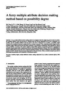
For the second step of AFRS approach, we applied existing VRP model for evaluating the overall round-trip delivery cost from the depot to all customers in each group under the constraint of truck capacity or the Capacityconstrained VRP (CVRP) [38]-[41]. In the next section, the proposed FMODM model is applied to the practical real world application. V. A CASE STUDY In order to illustrate the effectiveness of the proposed model for AFRS, a case study of the distribution problem of a medical equipment production company in Thailand is shown. For every week, five to six thousand goods which are stored in two available depots should be sent to fortytwo customers by 1,440 pieces-capacity trucks. Moreover, in the future these trucks may be replaced by 3,360 piecescapacity trucks. So, two types of truck capacity are considered. The package size for all customers is the same in all categories of goods. So, the truck can carry a multiple commodity in each round-trip travel to serve customers. The approximately evaluated transportation cost is 38.85 Thai Baht/Kilometer (THB/km). In conventional approach, customers are assigned to depots using the simple transportation cost model in the first stage of AFRS. Fig.2 depicts the result from this model. The location map of the two depots and the forty-two customers is shown. The customers represented by triangle are served by depot 1 and the customers represented by circle are assigned to depot 2. After routing using VRP, the total cost of transportation is calculated to be 13,595.56 THB per week when transported by 1,440 pieces-capacity trucks and 11,800.30 THB per week when transported by 3,360 piecescapacity trucks. From Fig.2, although all customers represented by triangle are close to depot 1 than depot 2, there are nine customers served by depot 1 (locate in the south of depot 1 in Fig.2), which should be assigned to depot 2 because they are in the vicinity of customers which are assigned to be served by depot 2. To apply the proposed FMODM model, firstly the relationship of all forty-two customers is evaluated using pairwise comparison as mentioned in Section III. For setting the goal, PIS of each objective is used. So the first goal is set to 27,240.45 THB and acceptable allowance of the first goal is 30,474.33 THB. Similarly, the second goal is set to 2,512 and acceptable allowance of the second goal is 3,892. In the proposed model, DM can design the acceptable satisfactory level, by assigning an aspiration level of both goals. In this case, an aspiration level of the first goal is set to 0.8. Then, the mathematical expression of the proposed FMODM model for this problem can be shown as follows, lex max = [λ1 ,λ 2 ], subject to
λ1 + δ1- − δ+1 =0.8, ⎛ z − 27,240.45 ⎞ λ1 ≤ 1 − ⎜ 1 ⎟, ⎝ 30,474.33 ⎠ ⎛ z − 2,512 ⎞ λ2 ≤ 1 − ⎜ 2 ⎟, ⎝ 3,892 ⎠ 2 42
+ ∑ ∑ cij dij xij + 30,474.33(δ1 − δ1 ) = 27,240.45, i
j
ISBN: 978-988-18210-5-8 ISSN: 2078-0958 (Print); ISSN: 2078-0966 (Online)
2 42
+ ∑ ∑ Qli xij + 3,892(δ2 − δ2 ) = 2,512, where l=j. i j
2
∑ xij = 1,
for all j.
i
42
∑ xij b j ≤ 4,000,
for all i .
xij = 0 or 1,
for all i and j.
j
δ1- ,δ+1 ,δ-2 ,δ+2 ≥ 0, δ1- δ+1 ,δ-2 δ+2 = 0, λ1 ,λ 2 ∈ [0,1]. X XX
is the customer served by depot 1 is the customer served by depot 2
1
3 2
4
8
5
9 12 6
Depot1
7
10
11
14
13
15
22
23 24
17
16
25 26
32
21 20
31
27
18 28
33
19
29 34
30 35
36 37
38
39
42 40
41
Depot2
Fig.2 The current location map of the case study
Fig.3 The improved location map of the case study
After applying the proposed model to the first step of AFRS, the solution of assigning customers to depot is different from conventional approach. Fig.3 shows the result of the proposed model. Nine customers who used to be served by depot 1 (locate in the south of depot 1 in Fig.2) are changed to be served by depot 2. After routing using VRP, we found that the total delivery cost is 13,128.19 THB IMECS 2010
Proceedings of the International MultiConference of Engineers and Computer Scientists 2010 Vol III, IMECS 2010, March 17 - 19, 2010, Hong Kong [6]
per week, which is reduced 467.37 THB per week when transported by 1,440 pieces-capacity trucks and 10,704.73 THB per week, which is decreased 1,095.57 THB per week when transported by 3,360 pieces-capacity trucks. Yearly delivery cost can be summarized in Table III.
[7]
Table III Yearly delivery cost after applying different assignment methods to the first step of AFRS
[9]
Approach Yearly delivery cost, THB TP model 706,969.12 [a], 613,615.60 [b] Proposed model 682,665.88 [a], 556,645.96 [b] Note: [a] : transported by 1,440 pieces-capacity trucks [b] : transported by 3,360 pieces-capacity trucks
Table IV The required computational time (in hh:mm:ss) in each step of AFRS using different assignment methods Approach Step1:Assignment Step2:Routing (VRP) TP model 48:00:00 [a], >24:00:00 [b] Proposed model