graph using the eigenvector associated with the second smallest eigenvalue of a ...... 26.1. 12 nan512. 74752. 522240. 71.2. 683. 23.0. 19 gearbox. 107624.
A Graph Based Davidson Algorithm for the Graph Partitioning Problem Michael Holzrichter Sandia National Laboratories Albuquerque, NM 5800, USA
and Suely Oliveira Dept. of Computer Science, The University of Iowa, Iowa City, IA 52242, USA Received (received date) Revised (revised date) Communicated by Editor's name ABSTRACT The problem of partitioning a graph such that the number of edges incident to vertices in di�erent partitions is minimized, arises in many contexts. Some examples include its recursive application for minimizing ll-in in matrix factorizations and loadbalancing for parallel algorithms. Spectral graph partitioning algorithms partition a graph using the eigenvector associated with the second smallest eigenvalue of a matrix called the graph Laplacian. The focus of this paper is the use graph theory to compute this eigenvector more quickly. Keywords: Graph Partitioning Algorithms, Spectral Algorithms, Fiedler Vector, Eigenvalue solvers
1. Introduction The problem of partitioning a graph such that the number of edges incident to vertices in di�erent partitions is minimized arises in many contexts. For example, the nested dissection algorithm [13] uses a solution to the graph partitioning problem to nd permutations of sparse matrices which reduce ll-in. Graph partitioning has been used in many other applications such as VLSI design and load-balancing for parallel algorithms. Spectral algorithms partition a graph based on the Fiedler vector, which is the second smallest eigenvector of a matrix, called the \graph Laplacian", associated with a graph. Finding this eigenvector represents the majority of the time required by spectral partitioning techniques. Fiedler [11, 12] did pioneering work on the relationship between the properties of a graph and the the Fiedler vector. Pothen, Simon, and Liou [26], explored the usage of the Fiedler vector for partitioning graphs. Hendrickson and Leland [17] generalized spectral bisection to perform quadrasection and octasection by using the third and fourth smallest eigenpairs of the graph Laplacian. Spielman and Teng [30] present an upper bound on the Fiedler value of bounded degree d-dimensional graphs, and they relate this upper bound to the number of edges cut by a Fiedler cut. 1
In this paper we apply graph theory to improve the computation of the Fiedler vector. In our new approaches the eigensolver is the Davidson algorithm, which is a subspace method allowing the use of preconditioners. The use of the Davidson algorithm for graph partitioning has not previously appeared in the literature. We modify the original Davidson algorithms to incorporate information about the graph in the form of a preconditioner. In addition, we use information about the graph to develop e�cient implementations. In other words, the original Davidson algorithm is modi ed in three ways: First, a series of coarse graphs is used as a framework for a multilevel preconditioner. Second, a favorable initial subspace for the Davidson algorithm is obtained by running the Davidson algorithm on the next coarser graph. Third, the series of coarse graphs were used to permute the input matrix to increase the concentration of the non-zero entries along the diagonal (this increased temporal and spatial locality of reference while computing the Fiedler vector). The Fiedler vector has proven to be useful for more than graph partitioning. Recent work uses the Fiedler vector to impose a total reorder rather than just a partition. This has been found to be useful for two closely related problems, envelope reduction and seriation. Envelope reduction [2, 14] attempts to minimize the maximum distance of non-zero elements from the diagonal. Atkins, Boman, and Hendrickson [1] discuss the seriation problem, which is to reorder a set of elements such that closely coupled elements appear as near as possible to each other in the new ordering.
2. Spectral Methods 2.1. The graph Laplacian Every undirected graph can be represented by an adjacency matrix. Similarly, every graph can be associated with a similar matrix, called its graph Laplacian. Spectral partitioning methods partition a graph using the second smallest eigenvector of its graph Laplacian (also known as Fiedler vector). Many properties of the graph Laplacian are discussed in [6, 32]. Let A be the adjacency matrix associated with a graph and D be a matrix such that all entries are zero except along the diagonal where di;i is equal to d(vi ), the degree of vertex vi . The graph Laplacian L is de ned as D ? A, i.e., in other words the elements of L are given by li;j = d(vi ) if i = j , ?1 if i 6= j , and the graph has an edge (vi ; vj ), and 0 otherwise. There is a one-to-one correspondence between vertices and elements of the Fiedler vector. A graph can be bisected by nding the median element of the Fiedler vector and then assigning vertices to one partition or another based on whether the corresponding element in the Fiedler vector is larger or smaller than the median. A similar process is used for other types of cuts such as \ratio cuts" by choosing another element instead of the median.
2
2.2. The Davidson's Eigensolver Many algorithms have been developed for computing eigenvalues and eigenvectors. General surveys of these techniques can be found in [8, 15, 25, 28]. In our work we introduce Davidson-type algorithms [4, 7, 24] as a basis for graph partitioning algorithms. Furthermore, we use graph theory to incorporate information about the problem into the Davidson eigensolver. Davidson-type algorithms are iterative subspace methods for nding a limited number of eigenpairs. They build up a set of orthogonal vectors which span nested subspaces of increasing dimension. Each iteration adds an additional basis vector, increasing the dimension of the subspace by one. A new basis vector is created by multiplying the residual by preconditioner M� and orthogonalizing the result against the existing basis vectors. If the identity were used as the preconditioner, Davidson's subspaces would be Krylov spaces and Davidson's algorithm would be equivalent to the Lanczos algorithm with reorthogonalization. The Davidson algorithm, like the Arnoldi algorithm, works well for non-symmetric matrices while the Lanczos algorithm is for symmetric matrices only. The pseudo-code for Davidson's method for computing the smallest eigenpair follows:
Algorithm 1 { Basic Davidson's Algorithm
Given matrix C , iteration limit m, and convergence factor �, compute eigenpair �, u. 1. Choose an initial vector v1 . Normalize v1 and make the result the sole column of V1 . 2. For j = 1; 2; : : : ; m or convergence do: (a) Compute w := Cvj . (b) Compute VjT w, and make this the last column and row of Sj where Sj = VjT CVj . (c) Compute the smallest eigenpair �~, y of Sj . (d) Form the Ritz vector u~ := Vj y. (e) Compute the residual r := C u~ ? �~u~; exit loop if krk < �. (f) Compute t := M� r. (g) Orthogonalize t against the columns of Vj to form vj+1 . Append vj+1 to Vj to form Vj+1 . 3. Return eigenpair �, u where � = �~ and u = u~. 2.3. Multilevel Graph Bisection Recently multilevel algorithms for partitioning graphs have been an area of active research [3, 16, 21]. Multilevel algorithms work with the graph at multiple levels of granularity. Increasing levels of granularity are obtained by combining adjacent vertices into \composite" vertices at the next coarser level of granularity. This maps the graph into another graph with fewer vertices. Connectivity of the original graph
3
is preserved by ensuring that two vertices at level k are connected by an edge if, and only if, there exists one or more edges between vertices at the next ner level which were combined to form the vertices at the coarse level. The process of coarsening a graph by combining pairs of adjacent vertices is repeated until a graph is obtained with su�ciently few vertices that another partitioning algorithm can quickly nd a high-quality partition. An initial partition for the coarsest graph is interpolated back onto the graph at the next ner level. After interpolation, the partition may be improved using a local re nement algorithm and the interpolation is repeated until the original ( nest) level of the graph has been reconstructed. The basic outline of this class of multilevel partitioning algorithms is 1) Coarsen the graph until the number of vertices is su�ciently small. 2) Partition the graph at the coarsest level, and 3) Uncoarsen and re ne the partition level by level until a partition of the original graph is obtained. There are a variety of choices for each of these steps. Karypis and Kumar explore many choices in [21]. To construct the next coarser graph Gi+1 from graph Gi , a maximal matching (maximal with respect to inclusion, not size) is found for Gi . A maximal matching for a graph is not unique. Karypis and Kumar construct maximal matchings by visiting the vertices of a graph in some order. If the vertex is adjacent to one or more unmatched vertices, then one of the unmatched neighbors is chosen to be paired with the visited vertex. If the vertex has no unmatched vertices, it is simply copied to the next coarser graph. Once all the vertices have been visited, a maximal matching will have been found. The coarse graph Gi+1 can be constructed from the ne graph Gi by combining the matched vertices. Provided the coarsest graph is su�ciently small, a wide range of partitioning methods, including spectral partitioning, can quickly nd a high quality partition of the coarse graph. The time required to partition the coarse graph becomes a minor consideration and the partitioning technique can be chosen based on the characteristics of the partition produced. Variations of the Kernighan-Lin algorithm [22] are widely used for this step. Spectral techniques (usually based on the Lanczos algorithm) have been employed to partition the coarsest graph. When a partition is interpolated onto the next ner graph, the result is a partition which is not optimal for that graph. That partition is re ned after interpolation. A variation of Kernighan-Lin called \Boundary Kernighan-Lin" (BKL) can be used to re ne the graph. BKL is e�cient during the re nement phase because it restricts the pairs of vertices considered for swapping to those which lie along the boundary between the two partitions. This signi cantly speeds the re nement step.
3. New Methods In the previous section, we mentioned that traditional spectral partitionings (such as Lanczos algorithm for example) are only applied to the coarsest representation of the graph. Because our algorithms are cheaper than the Lanczos, they make it possible to perform spectral partitioning of the original graph. In addition, they are not coupled with other heuristic algorithms. Our methods are purely 4
spectral methods. Multilevel algorithms nd a partition for an input graph G0 by working with additional graphs G1 ; G2 ; : : : Gn , constructed by successive coarsening of G0 . Previous multilevel graph partitioning algorithms worked by transforming an initial partition of the coarsest graph Gn into a partition for G0 by interpolation onto successively ner graphs followed by local re nement. The key feature of the new approaches presented here is that, rather than partitioning the coarsest graph Gn , information about the graph's structure provided by fG0 ; G1 ; : : : ; Gn g is used to accelerate the computation of the Fiedler vector for the input graph. Due to the method used to construct them, vertices of a coarse graph Gj represent highly connected regions of G0 . The size of the region of G0 represented by a vertex of Gj increases with j , i.e. increases with the coarseness of the graph. Thus, the series of graphs fG0 ; G1 ; : : : ; Gn g are one kind of representation of the graph's structure. Our new algorithms use the information about the graph's structure represented by fG0 ; G1 ; : : : ; Gn g in novel ways. The rst two new methods (Sections 3.1 and 3.2) we will present achieves the goal of reducing the number of iterations required to nd the Fiedler vector. The third new method (Section 3.3) enhances the implementation of the eigensolver by reordering the data structures in memory to increase spatial and temporal locality, improving the e�ectiveness of the computer's cache memory. We call the resulting method when one or more of these algorithms are used and applied to the input graph, \Multilevel Davidson Algorithm" (MDA). 3.1. Preconditioned Davidson Algorithm (PDA) One property of graph Laplacian matrices is that the smallest eigenvalue is always 0 and the corresponding eigenvector is the vector (1; 1; : : : ; 1)T . Based on this a priori knowledge, the initial set of basis vectors is augmented with an additional basis vector - the unit vector in the direction of (1; 1; : : : ; 1)T . Due to the size of L, solving Lti = ri can be expensive. We developed an algorithm for solving this system based on graphs fG0 ; G1 ; : : : ; Gn g. This gives us a framework for a multilevel preconditioner for solving Lti = ri . Multilevel iterative methods have proven to be e�ective for solving systems of linear equations arising from PDE's [5, 23]. While the traditional multilevel approach for solving elliptic PDE's obtains smaller problems by coarsening the spatial discretization, our Preconditioned Davidson Algorithm implements a preconditioner which uses fG0 ; G1 ; : : : ; Gn g as its multilevel framework. This preconditioner can be used on irregular matrices arising from unstructured graphs where the usual coarsening process is ill-de ned or not applicable. Let G0 , be the input graph which has been successively coarsened to form G1 to Gn . Let Lj be the graph Laplacian associated with graph Gj and r0 be the residual at the end of the ith iteration. (The iteration index i is implicit since one application of the preconditioner begins and ends in the same iteration of the Davidson algorithm.) The restriction of r0 onto graph Gj is rj . The basic idea behind the multilevel preconditioner is to use relaxation to nd an approximate
5
solution tj to Lj tj = rj . Projecting this solution onto the next ner graph Gj?1 provides a good starting point for performing relaxation to nd tj?1 which is a solution to Lj?1 tj?1 = rj?1 . The new multilevel preconditioner, expressed as pseudocode, follows:
Algorithm 2 { Multilevel Preconditioner for Laplacian System Given residual vector r , graphs fG ; G ; : : : ; Gn g, graph Laplacians fL ; L ; : : : ; Ln g, and relaxation count parameters n and n , compute 0
0
0
1
1
1
2
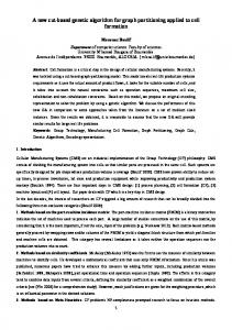
vector t0 , which is an approximate solution to L0 t0 = r0 . 1. Compute fr1 ; : : : ; rn g by successively restricting r0 to graphs G1 ; G2 ; : : : ; Gn . 2. Find tn which solves Ln tn = rn . 3. For i = n ? 1; n ? 2; :::0 do (a) Create ti by interpolating ti+1 onto graph Gi . (b) Set yi = ri . (c) For j = i; i + 1; : : : ; n do i. Relax n1 times the system Lj tj = yj using Gauss-Seidel. ii. Form yj+1 by computing the residual Lj tj ? yj and restricting onto graph Gj+1 . (d) Find tn which solves Ltn = yn . (e) For j = n ? 1; n ? 2 : : : ; i do i. Interpolate tj+1 onto graph Gj and sum with existing tj . ii. Relax n2 times the system Lj tj = yj using Gauss-Seidel. 4. Return t0 as an approximate solution to L0 t0 = r0 . Figure 1 illustrates our multilevel preconditioner for a graph which has been coarsened to four levels. Figure 1 shows the path though the di�erent levels of graphs and the operations performed along the way. The process is very similar to full multigrid V-cycles, but di�ers by using graph theory to de ne the restriction and interpolation operations. The circles, squares, triangles, and hexagons represent an operation using the graph at that level as input. The action represented by the di�erent shapes are:
� Circle - solve Lntn = yn on the coarsest graph. This is steps 2 and 3-d in
the pseudocode. � Square - interpolate ti+1 found for graph Gi+1 onto graph Gi to form ti . This is steps 3-a and 3-b in the pseudocode. � Triangle - interpolate tj+1 onto graph Gj and sum with existing tj then relax Lj tj = yj n2 times using Gauss-Seidel. This is step 3-e in the pseudocode. � Hexagon - relax Lj tj = yj n1 times using Gauss-Seidel then restrict the residual Lj tj ? uj onto graph Gj+1 to form yj+1 . This is step 3-c in the pseudocode. 6
Level 0: Level 1: Level 2: Level 3: Solve Ltn = yn on coarsest graph Interpolate ti+1 onto graph Gi to form ti Interpolate tj+1 onto Gj and sum with existing tj then relax n2 times Relax Ljtj = yj n1 times then restrict residual onto graph Gj+1 to form yj+1
Figure 1: Operation of multilevel preconditioner for four graph levels 3.2. Nested Davidson Algorithm (NDA) The Nested Davidson Algorithm generalizes the Davidson algorithm by allowing the use of multiple vectors for the initial subspace. Advantageous basis vectors for G0 are obtained by performing Davidson on G1 , the next coarser graph and interpolating linear combinations of the basis vectors for G1 onto G0 then reorthogonalizing. The assumption is that basis vectors for G1 will yield favorable basis vectors when interpolated onto G0 such that the distance between the Fiedler vector and its interpolation into the subspace is small. Moreover, multiple bases allows more degrees of freedom when approximating the Fiedler vector. The same approach can be used to accelerate the Davidson algorithm on G1 making NDA a recursive algorithm. The recursion terminates with the coarsest graph, Gn . Linear combinations of the resulting basis vectors are interpolated onto the next ner graph Gn?1 to create an initial subspace as a starting point for NDA on Gn?1 . The process works its way up the hierarchy of graphs until the Fiedler vector for the nest graph G0 has been computed. The Nested Davidson Algorithm and Barnard and Simon's Multilevel Spectral Bisection (MSB) [3] both nd the Fiedler vector for ner and ner graphs using the interpolation of the result from the next coarser graph as a starting point for the current graph. While MSB uses the Rayleigh Quotient Iteration to re ne the newly interpolated Fiedler vector, NDA interpolates basis vectors onto the ner graph and uses them as a set of basis vectors for the initial subspace of our PDA algorithm. The Nested Davidson Algorithm modi es the Davidson algorithm in the following way:
7
First, before the Fiedler vector is computed for Gj , NDA recursively computes the Fiedler vector of the next coarser graph, Gj+1 . The recursion yields l basis vectors for Gj+1 . These basis vectors are interpolated onto Gj and then reorthonormalized. These vectors become the basis for the initial subspace for the Davidson algorithm applied to the graph Laplacian of Gj . The l basis vectors passed to the caller are weighted sums of the k basis vectors for the subspace constructed at the current level of recursion. Let fa0 ; a1 ; : : : ak g be the weights of the expansion of the Fiedler vector at level j + 1 in terms of the basis vectors for that level. Let s(i) be a function which gives the index of the weight with the ith largest magnitude. l vectors fb0; b1 ; : : : bl?1 g are formed from the k basis vectors fv0 ; v1 ; : : : vk?1 g according to the formula:
bi =
p X j =0
as(i+l�j) vs(i+l�j) where p =
�
bk=lc + 1 if i < k mod l bk=lc otherwise.
This creates l vectors from the k basis vectors such that the Fiedler vector is a linear combination of these l new vectors. These vectors fb0 ; b1 ; : : : bl?1 g are interpolated onto Gj and reorthogonalized. The pseudocode for the Nested Davidson Algorithm is:
Algorithm 3 { Nested Davidson Algorithm Given graphs fGi ; Gi ; : : : ; Gn g, graph Laplacians fLi ; Li ; : : : ; Lng, +1
+1
iteration limit m and maximum dimension of initial subspace l, compute eigenvector x and B , whose l columns are linear combinations the columns of V such that x lies in the subspace spanned by the columns of B . 1. Set v0 := (1; : : : ; 1)=k(1; : : :; 1)k. 2. Set S0;0 := v0T Lj v0 . 3. If current graph is Gn then (a) Choose arbitrary v1 and normalize. Otherwise (b) nested davidson(Gj+1 ; B ) (c) For k = 1 to l do: i. Interpolate bk?1 onto graph Gj and orthogonalize against columns of Vk?1 to form vk . Append vk to Vk?1 as the last column to form Vk . ii. Compute Vk Lj vk and make the result the last row and column of S . 4. For k = l; 2; : : :; m + l ? 1 or convergence do: (a) Perform Davidson iterations. 5. Return vk as x. Construct l vectors from linear combinations of the k current basis vectors and store them as the columns of B . 8
More details about NDA are presented in [19, 18]. 3.3. Multilevel Graph Reordering (MGR) Graph Laplacian matrices are stored in memory using large, irregular data structures. These data structures may result in memory access patterns with poor temporal and spatial locality, thereby harming performance. Multilevel Graph Reordering (MGR) is a heuristic we use to reorder the storage of graph data structures to improve the bene t of cache memories when performing the PDA and NDA algorithms. Douglas [10] studied ways to modify multigrid algorithms so that their memory access patterns take better advantage of cache memory. Douglas' solution is predicated upon regularity in the discretization of the problem. The PDA and NDA algorithms do not assume any regularity in the structure of the input matrix so Douglas' techniques are not applicable. Toledo [31] discussed locality of reference when performing LU decomposition. MGR addresses a problem distinct from those considered by Douglas, namely the locality behavior of PDA and NDA when used on graphs of unknown or irregular structure. Pothen and Ye have presented preliminary results for reordering data access in a irregular mesh for an Euler Equation solver [27]. Their reordering data accesses include Cuthill-McKee, Sloan, Nested Dissection, and space- lling-curve algorithms and are disctinct from the method we present below. MGR attempts to enhance locality by permuting the graph Laplacian matrices in a manner which concentrates the non-zero entries near the diagonal. Concentrating non-zero elements along the diagonal improves locality of memory references during relaxation, which is the major time consuming step in our calculation of the Fiedler vector. In addition to permuting the matrix, the data structures are rearranged in memory. This was necessary because the random order in which vertices are visited during coarsening resulted in data structures with non-contiguous indices stored contiguously in memory. The order of edges in the edge list were sorted into increasing order also. As a result, vertices with contiguous indices were stored in data structures with contiguous memory addresses. The graphs fG0 ; G1 ; : : : ; Gn g provide the means to nd a permutation which increases the density of non-zero elements along the diagonal quickly and e�ciently. Our MGR implementation extended fG0 ; G1 ; : : : Gn g with additional coarse graphs until a graph with a single vertex was obtained. A tree was imposed on the vertices. (The edges of the graphs were ignored during the relabeling process.) The children of a vertex in graph Gj are the vertices of Gj?1 which were combined to form that vertex. The result is a tree spanning all vertices in fG0 ; G1 ; : : : Gn g. Renumbering was accomplished by visiting the vertices in a depth- rst traversal of the tree. A vertex of graph Gj was assigned an index of i if it was the ith vertex of Gj to be visited in the depth- rst traversal. Figure 2 illustrates a sample tree for a graph with four levels. In this gure, solid lines represent parent/child relationships in the tree and dotted lines indicate
9
Level 3:
A
B
Level 2:
Level 1:
C
D
G
Level 0:
F
E
I
H
J
Figure 2: Storage of data structures before reordering the path of the depth- rst traversal during reordering. A vertex's memory address relative to other vertices in the same graph is indicated by its horizontal position. If a vertex is to the left of another vertex in the same level then it is stored at a lower memory address. The result of rearranging the storage of vertices in Figure 2 using MGR is illustrated in Figure 3. The depth- rst traversal visited vertex B and its descendants E, G, and J before vertex C and its descendants. As a result B and its descendants appear to the left of C and its descendants re ecting their placement at lower memory addresses. The pseudocode for MGR follows:
Algorithm 4 { Multilevel Graph Reorder Given fG ; G ; : : : Gn g, nd permutation of graph Laplacian L which 0
1
concentrates non-zero entries near the diagonal.
0
1. Extend fG0 ; G1 ; : : : Gn g with additional coarse graphs until a graph with a single vertex is obtained. 2. Using mapping of vertices in Gj to vertices of Gj+1 construct tree such that vertices of Gj are children of vertices of Gj+1 . 3. Traverse tree in depth- rst manner. Assign new index to each unvisited node. An index i is assigned to a vertex of graph Gj if it is the ith vertex of Gj to be visited during the depth- rst traversal of the tree. 4. Update data structures to re ect new order: 10
Level 3:
A
B
Level 2:
Level 1:
Level 0:
C
E
G
F
D
I
J
H
Figure 3: Storage of data structures after reordering
� Update contents of data structures to re ect new indices as-
signed to vertices. � Reorder data structures in memory such that data structures corresponding to vertex v0 have lowest memory addresses followed by data structures for v1 and so on. � Sort the edge list of vertices. For the complexity analysis of the above algorithms, we assume k0 to be the number of iterations at the nest level, jV j the number of vertices, and jE j the number of edges. In analyzing the time complexity of MDA, it is useful to break down the overall time into the time spent performing calculations at each level. The operations performed by the preconditioner with the greatest time complexity are relaxations. The time complexity of a single relaxation at level i is proportional to jEi j, the number of edges of Gi . During the coarsening process, intermediate graphs were removed to ensure a minimum ratio of the number of vertices at level i to the number of vertices at i + 1. Let r be the value of this ratio and require r > 1 (r = 4 for the experiments in this paper). Assume that a similar ratio holds for the number of edges. The time for a relaxation, interpolation or restriction at level i is bounded by C jEi j. Since level i is part of i + 1 V-cycles, the amount of time spent performing operations on level i is bounded by C 0 (i + 1)jEi j for some constant C 0 . Thus the total time for the operations at all levels is Total time � C 0
#X levels (i + 1)jEi j: i=0
11
Since jEi+1 j � (1=r)jEi j, the total time is bounded by
C0
#X levels 1 1 1 2 X 0 0 r jE0 j: ( i + 1) j E j � C ( i + 1) j E 0 0j = C i i r r (r ? 1)2 i=0
i=0
Provided r > 1 is bounded away from one, the total time is linear in jE0 j = jE j. The space complexity of MDA is O(jV j). For the complexity analysis of NDA, we assume the number iterations at level i is O(k0 ) where k0 is the number of iterations required by NDA at level 0, the nest level. Matrix-vector multiplications each require O(jEi j) time and orthogonalizing a vector against m orthonormal vectors requires O(mjVi j) time. An O(k3 ) QR method was used to nd the eigenpairs of the dense matrix in the Rayleigh-Ritz process. Since, at a given level, this was done once for k = 1; 2; : : :O(k0 ), solving the eigenpairs for the projection into the subspace involved O(k04 ) work. At level i, O(k0 ) iterations of the Davidson algorithm are performed requiring a total of O(k0 jEi j), O(k0 jEi j), O(k02 jVi j), and O(k04 ) time for multilevel preconditioning, matrix-vector multiplication, orthogonalization, and Rayleigh-Ritz' eigenproblem, respectively. The total time complexity of NDA at level i is O(k0 jEi j + k02 jVi j + k04 ). Since NDA is run once for each level, the total P by NDA for all levels can be P time required jVi j and jVi+1 j found by summing over i to give O(k0P i jEi j + k02 i jVi j + k04). Since P , i.e. i jVi j = O(jV j). satisfy a minimum ratio r, the sum i jVi j is linear in jV jP Assuming that the edges also satisfy a similar ratio gives i jEi j = O(jE j). The overall time complexity of NDA becomes O(k0 jE j + k02 jV j + k04 ). NDA computes the Fiedler vector at level i +1 before performing any signi cant computation at level i. The space required for the recursion can be reclaimed before allocating space for the current level. Whereas the regular Davidson algorithm starts with a single basis vector, NDA allows for as many as l. Typically O(ljV j) additional storage is required to accommodate the additional l ? 1 basis vectors. NDA can be run in a mode in which all basis vectors at level i + 1 are interpolated onto level i and used to seed the Davidson algorithm. Not only are all basis vectors from level i + 1 interpolated onto level i, but every iteration at level i adds an additional basis vector. The number of bases for level i is the cumulative total created for that level and all coarser levels. Assuming convergence after O(k0 ) iterations, each of the O(log jV j) levels will contribute O(k0 ) basis vectors, each of length jV j. In this case O(k0 jV j log jV j) storage will be required. Multilevel Graph Reordering has two phases. The rst phase relabels the vertices of a graph and the second phase reorders the data structures based on that relabeling. The coarsening process gives rise to a tree involving vertices of the graphs G0 ; G1 ; : : : ; Gn . The parent-child relationship of the tree re ects which vertices of Gi?1 were combined to form a vertex in Gi . The tree is a by-product of the coarsening process and does not increase the complexity of Multilevel Graph Reordering. Relabeling the vertices is accomplished via a depth- rst traversal of this tree. Relabeling entails a constant amount of work at each vertex visited in the traversal, therefore the time complexity of relabeling is that of the depth- rst 12
traversal, O(jE j + jV j), or O(jE j) under the assumption that the graph is connected because jE j will be at least jV j ? 1. The reordering phase of Multilevel Graph Reordering was implemented as a three step process - a copy of all vertex and edge data structures were made, the data was copied back into the original memory in the new order, and then the edges for each vertex were sorted into increasing order. Moving the data structures to and from temporary bu�ers entailed a constant amount of work for each vertex and edge as did the update of the contents to re ect the relabeling. Sorting the edges has the potential of being more time consuming. In the general case, sorting Ev , the set of edges for vertex vi has O(jEv j log jEv j) time complexity, making the reordering phase O(jV j2 log jV j) in the worst case where jE j = O(jV j2 ). In practice, the graphs associated with large, sparse matrices typically have bounded degree. For bounded degree graphs, the time required to sort the edges for an individual vertex is O(1) and the reordering phase is O(jE j + jV j). Under the assumptions that a graph is connected and has bounded degree, the overall time complexity of Multilevel Graph Reordering is O(jE j). Again, in the worst case, Multilevel Graph Reordering is O(jV j2 log jV j). The implementation of Multilevel Graph Reordering used in this paper used a constant amount of auxiliary storage for each vertex and edge resulting in a space complexity of O(jE j + jV j). Doing so did not increase the overall space complexity of the program because O(jE j + jV j) storage was used to store the graph data structures in memory anyway. The amount of auxiliary storage can be reduced by reordering the data structures in place but O(jV j) storage is still required to store relabeling information. i
i
i
4. Numerical Experiments The e�ectiveness of PDA, NDA, and MGR were gauged by their performance partitioning a suite of test cases. We used the Metis software of Kumar and Karypis, as a framework for our new algorithms. The Metis software provided useful data structures and supporting functionality such as graph coarsening, le IO and timing facilities. For more information about our codes, please refer to [18, 19]. The tests were conducted on an SGI Origin 2000 with 8 gigabytes of RAM and 250 MHz R10000 CPUs, each with 4 megabytes of secondary cache. The tests were run in a dedicated environment. The Fiedler vector was found for the nest graph in all runs. A vector was deemed to have converged to the Fiedler vector when the l2 norm of the residual was less than 10?5. Graphs were coarsened using the Heavy Edge Matching strategy [21]. For all graphs, Gn (the coarsest graph) had at most 100 vertices. A 4:1 ratio was imposed on the number of vertices in Gj and Gj+1 by removing intermediate graphs as necessary. The suite of test cases were obtained by extracting graphs from large, symmetric matrices from scienti c applications [9]. The matrices used in the experiments range in size from 12,000 by 12,000 to more than 200,000 by 200,000. The number of edges ranges from approximately 300,000 to more than 11 million. The test cases 13
Table 1: Performance of Lanczos and MDA Algorithms Graph Vertices Edges 3dtube 45330 3168288 bcsstk31 35586 1145826 bcsstk32 44609 1970092 bcsstk35 30237 1419926 cfd1 70656 1757708 cfd2 123440 2964458 ct20stif 52329 2646134 nan512 74752 522240 gearbox 107624 6500976 nasasrb 54870 2622454 pwt 36463 289588 pwtk 217918 11416506
Lanczos Lanczos Davidson Davidson Time Iterations Time Iterations 89.8 236 46.8 20 64.2 437 17.9 18 118.5 482 26.6 17 65.5 377 21.4 20 76.4 313 29.0 16 153.4 367 62.3 20 126.8 390 26.1 12 71.2 683 23.0 19 501.4 636 453.3 87 95.9 296 40.0 20 30.1 693 8.6 19 1139.5 807 378.1 42
come from diverse problem domains ranging from nancial portfolio optimization methods to sti�ness matrices for automobile components. The performance of the new algorithms were explored through a series of four numerical experiments. These experiments assess the new algorithms when used individually (Sections 4.2,4.3 and 4.4) and in combination (Section 4.1). 4.1. Collective Performance of MDA vs. Lanczos The rst experiment tests the overall e�ectiveness of MDA (PDA+NDA+MGR) against the widely used Lanczos algorithm. Numerical data from this experiment are shown in Table 1. The table lists the time, in seconds, and the number of iterations required to obtain the Fiedler vector. The time required by the new algorithms is considerably less than that of Lanczos for all graphs in the test suite. Figure 4 shows the ratio of the time required by the modi ed Davidson algorithm to the time required by the Lanczos algorithm. All values are less than 1.0 indicating that MDA was faster for all of these graphs. Most values are between 0.3 to 0.5 indicating that MDA is usually 2 to 3 times as fast. MDA was as much as 5 times as fast for the graphs bcsstk32 and ct20sti�. Only the gearbox graph had a ratio signi cantly more than 1:2. Figure 5 shows the l2 norm of the residual versus iteration number for MDA. The plot has one data point for each iteration for each graph. The plot shows that all but two of the graphs converged at a similar rate. The norm of the residual of these graphs decreased by roughly one order of magnitude every six iterations. The graphs pwtk and gearbox showed anomalously slow convergence. Pwtk started o� converging at a rate comparable to that of the other graphs but slowed considerably after ten iterations. Gearbox exhibited slow convergence from the start. The residual of gearbox decreased roughly one order of magnitude for each
14
3dtube bcsstk31 bcsstk32 bcsstk35 cfd1 cfd2 ct20stif finan512 gearbox nasasrb pwt pwtk 0.0
0.2
0.4
0.6
0.8
1.0
Figure 4: Ratio of MDA to Lanczos execution time twenty iterations. The Lanczos and MDA algorithms are two methods for nding the same vector. It was not surprising that the number of edges cut for eight out of twelve graphs was identical whether Lanczos or MDA was used to nd the Fiedler vector. The di�erence in edge cut was one for bcsstk32. Lanczos produced a slightly better edge cut for cfd1 (9969 vs. 10046 edges). MDA produced a slightly better edge cut for gearbox (29710 vs. 29767 edges). MDA produced a signi cantly better cut for ct20sti� (17174 vs. 18287 edges). When the di�erence in edge cut is small (less than 10), it is likely that the partitions are almost identical except for one or two vertices assigned to di�erent partitions. This can be caused by small di�erences in the individual entries of the Fiedler vector. When the di�erence is large, the di�erence in edge cut can be attributed to convergence to nearby but distinct eigenpairs. 4.2. Componentwise Performance of MDA: Multilevel Preconditioner (PDA) The e�ectiveness of the multigrid preconditioner is explored by the this experiment. The performance of the multilevel preconditioner of PDA was assessed by comparing its performance against the diagonal preconditioner. The numerical performance of the diagonal preconditioner is not as good as the multilevel preconditioner but it is very fast. Table 2 presents the execution time, in seconds, and number of iterations. Using the multilevel preconditioner required both fewer iterations and less time to compute the Fiedler vector. For all but three graphs, using the diagonal preconditioner took four or more times as long as the multilevel preconditioner. The multilevel preconditioner gave a speedup of more than ten for some of the graphs. The reduction in the number of iterations was su�cient to compensate for the additional expense of the multilevel preconditioner.
15
10 "3dtube" "bcsstk31" "bcsstk32" "bcsstk35" "cfd1" "cfd2" "ct20stif" "finan512" "gearbox" "nasasrb" "pwt" "pwtk"
1
Norm of Residual
0.1
0.01
0.001
0.0001
1e-05
1e-06 0
10
20
30
40 50 60 Iteration Number
70
80
90
Figure 5: l2 norm of residual as a function of iteration number.
Table 2: Performance of Multilevel and Diagonal Preconditioners Graph 3dtube bcsstk31 bcsstk32 bcsstk35 cfd1 cfd2 ct20stif nan512 gearbox nasasrb pwt pwtk
Multilevel Multilevel Diagonal Diagonal Time Iterations Time Iterations 46.8 20 93.4 98 17.9 18 100.4 138 26.6 17 129.3 134 21.4 20 127.7 160 28.9 16 160.1 132 62.6 20 323.1 146 26.1 12 59.8 65 23.0 19 327.5 149 453.3 87 3010.0 398 39.9 20 77.7 86 8.8 19 196.6 203 378.9 42 4644.0 362
16
3dtube bcsstk31 bcsstk32 bcsstk35 cfd1 cfd2 ct20stif finan512 gearbox nasasrb pwt pwtk 0.0
0.1
0.2
0.3
0.4
0.5
0.6
Figure 6: Ratio of multigrid to diagonal preconditioner execution times Both the diagonal and multilevel preconditioners require approximately constant time per iteration but the time and space requirements of other parts of the Davidson algorithm increase with the number of iterations. For this reason, among preconditioners which perform a constant amount of work per iteration, there is an incentive to trade an increase in the complexity of the preconditioner for a reduction in the number of iterations. 4.3. Componentwise Performance of MDA: Nested Davidson Algorithm (NDA) The Nested Davidson Algorithm tries to speed the computation of the Fiedler vector of G0 by starting with a favorable initial subspace. Ideally, the component of the Fiedler vector perpendicular to the initial subspace is small. This experiment studied how well NDA provides a favorable initial subspace. The experiment compared the performance as a function of l, the dimension of the initial subspace, i.e. the number of basis vectors obtained from the next coarser graph. The value of l ranged from zero to unlimited. Zero represents the case where NDA is not used and unlimited represents the case where the subspace for Gj is initialized with all basis vectors from graph Gj+1 . Table 3 presents data from the second experiment. The elapsed time, in seconds, spent executing Davidson algorithm without NDA appear in the second column. NDA is represented by the remaining six columns. In the case where the initial subspace has just one basis vector, the basis vector is the Fiedler vector of Gj+1 . The times in the last column re ect the case where all basis vectors for Gj+1 are interpolated onto Gj to form the basis vectors of the initial subspace. Our results show that NDA indeed decreases execution time. While the improvement is often substantial, the amount of improvement is quite variable. Figure 7 shows the ratio of the times required by NDA divided by the time required without NDA. There is a general overall reduction in time when NDA is used and the improvement increases
17
Table 3: Performance of Nested Davidson Algorithm No 1 3 5 10 20 Bases Bases Bases Bases Bases Bases Graph Time Time Time Time Time Time 3dtube 52.5 40.8 43.5 44.0 47.2 47.7 bcsstk31 32.3 23.9 23.6 22.2 21.4 17.9 bcsstk32 67.5 52.4 51.6 52.4 33.7 26.6 bcsstk35 44.2 33.6 31.1 32.5 26.6 21.4 cfd1 88.0 55.4 51.5 49.4 41.2 29.1 cfd2 141.5 108.1 107.0 97.9 78.4 62.3 ct20stif 79.4 38.1 36.9 34.1 30.3 26.1 nan512 44.7 28.1 28.8 29.5 25.2 25.2 gearbox 488.3 450.9 444.1 428.9 432.8 453.5 nasasrb 76.7 55.4 39.8 44.0 36.5 40.0 pwt 42.6 21.2 14.0 13.2 11.4 8.6 pwtk 1009.8 673.0 669.3 770.8 615.7 378.9
All Bases Time 33.8 15.6 23.8 17.6 31.6 66.7 34.2 27.6 236.9 34.5 10.2 206.3
with the number of bases. For 20 bases, the average speedup approaches 2. One interpretation of the general improvement with the dimension of the initial subspace is that the additional dimensions represent degrees of freedom. The additional degrees of freedom give the Rayleigh-Ritz process ner control to emphasize certain directions and suppress others when computing the approximation to the Fiedler vector. Table 4 shows the inner product of the Fiedler vector with its projection in the initial subspace created by NDA for the various graphs. Since the Fiedler vector has unit length, the closer this value is to 1.0, the less the distance between the Fiedler vector and its projection. The majority of the entries have inner products in excess of 0.99 indicating NDA provides a very good initial subspace for the Rayleigh-Ritz process to search for the vector closest to the desired eigenvector. 4.4. Componentwise Performance of MDA: Multilevel Graph Reordering (MGR) The last experiment tests the e�ectiveness of the reordering technique. This experiment measured performance when Multilevel Graph Reordering was used against executions when no reordering or random reordering was used. The performance metric was cache line reusage. Cache line reusage is the average number of references made to a cache line before it is evicted from cache. Cache line reusage is one of the statistics output by the \perfex" performance monitoring utility of SGI computers. The R10000 chip has two counters which can be programed to count events such as memory accesses, cache misses etc. while executing the program at full speed. Perfex accesses these registers to compute a variety of statistics, including cache line reusage. Table 5 shows cache performance statistics. The value to the left of the slash is the average number of times a cache line in the primary cache was reused before being evicted and the number to the right is the average number of times a line in
18
1 Basis 3 Bases 5 Bases 10 Bases 20 Bases All Bases 0.0
0.2
0.4
0.6
0.8
1.0
Figure 7: Ratio of nested to non-nested Davidson algorithm execution times
Table 4: Inner Product of Fiedler Vector With Its Projection in Initial Subspace
Graph 3dtube bcsstk31 bcsstk32 bcsstk35 cfd1 cfd2 ct20stif nan512 gearbox nasasrb pwt pwtk
Second Finest Graph 0.30263 0.99784 0.99869 0.99799 0.99918 0.99933 0.99741 0.99861 0.78122 0.99980 0.99966 0.99970
19
Finest Graph 0.99174 0.99954 0.99982 0.99962 0.99973 0.99978 0.99961 0.99995 0.84086 0.99993 0.99994 0.99998
Table 5: Average Primary and Secondary Cache Line Reusage
Graph 3dtube bcsstk31 bcsstk32 bcsstk35 cfd1 cfd2 ct20stif nan512 gearbox nasasrb pwt pwtk
Multilevel Graph No Random Reorder Reorder Reorder (Prim. / Sec.) (Prim. / Sec.) (Prim. / Sec.) 13.9 / 5.3 11.2 / 6.6 9.8 / 7.8 11.8 / 6.4 9.9 / 6.8 9.4 / 8.3 12.6 / 5.7 10.9 / 6.2 10.2 / 6.8 12.4 / 5.7 10.9 / 6.6 9.6 / 7.9 10.5 / 6.2 8.5 / 7.7 7.2 / 9.4 10.4 / 5.8 7.9 / 7.5 7.1 / 8.0 14.1 / 5.4 10.9 / 6.8 10.1 / 7.5 7.7 / 9.0 6.1 / 10.5 5.8 / 11.0 11.2 / 5.2 9.2 / 6.4 8.0 / 7.0 12.5 / 5.4 11.0 / 6.2 10.1 / 7.1 8.3 / 10.7 6.4 / 12.9 6.5 / 12.8 11.8 / 4.6 9.6 / 5.8 8.7 / 5.5
the second level cache was reused. The data re ect the cache usage of the whole program rather than just the computation of the Fiedler vector. The data in Table 5 show that MGR had a de nite positive impact on improving hit rates for the primary cache. The average number of times a line in the primary cache was reused under MGR was 18% more than if no reordering was done.
5. Summary Spectral partitioning can be derived by casting the graph partitioning problem as a discrete optimization problem. The new algorithms presented here preserve the solution to the discrete optimization problem by nding the Fiedler vector of the input graph. However, the new algorithms use the multilevel representation of the graph provided by coarsening the graph to speed up the computation of the Fiedler vector. The Davidson algorithm was used to compute the Fiedler vector. Three new algorithms were developed to speed up the Davidson algorithm. The Preconditioned Davidson Algorithm used the multilevel representation of the graph as the framework for a multilevel preconditioner. The Nested Davidson Algorithm found a favorable initial subspace with which to start the Davidson iterations. Multilevel Graph Reordering used the multilevel representation to reorder the storage of the graph in memory to enhance locality of memory references. The Preconditioned Davidson Algorithm and Nested Davidson Algorithm proved to be quite e�ective at reducing the time required to nd the Fiedler vector for a range of graphs. Multilevel Graph Reordering met the goal of improving overall cache hit ratios. 20
Acknowledgements This research was supported by NSF grant ASC 9528912 and currently by NSF grant DMS 9996089. We thank the referees for advice which has improved the paper presentation. Part of this research was carried out in the Computer Science Department and Supercomputer Center of Texas A&M University.
References 1. J. Atkins, E. Boman, and B. Hendrickson. A spectral algorithm for seriation and the consecutive ones problem. SIAM Journal on Computing, 28:297{310, 1998. 2. S. Barnard, A. Pothen, and H. Simon. A spectral algorithm for envelope reduction of sparse matrices. Numerical Linear Algebra with Applications, 2:317{334, 1995. 3. S. Barnard and H. Simon. A fast multilevel implementation of recursive spectral bisection for partitioning unstructured problems. In Proceedings of the Sixth SIAM Conference on Parallel Processing for Scienti c Computing, Norfolk, Virginia, 1993. SIAM, SIAM. 4. L. Borges and S. Oliveira. A parallel Davidson-type algorithm for several eigenvalues. Journal of Computational Physics, (144):763{770, August 1998. 5. W. L. Briggs. A Multigrid Tutorial. Society for Industrial and Applied Mathematics, Philadelphia, Pennsylvania, 1987. 6. F. R. K. Chung. Spectral Graph Theory. American Mathematical Society, Providence, Rhode Island, 1997. 7. E. Davidson. The iterative calculation of a few of the lowest eigenvalues and corresponding eigenvectors of large real-symmetric matrices. Journal of Computational Physics, 17:87{94, 1975. 8. E. Davidson. Super-matrix methods. Computer Physics Communications, 53:49{ 60, 1989. 9. T. Davis. University of orida sparse matrix collection. March 1998. http://www.cise.u .edu/ davis/sparse/. 10. C. Douglas. Caching in with multigrid: problems in two dimensions. Parallel Algorithms and Applications, 9:195{204, 1996. 11. M. Fiedler. Algebraic connectivity of graphs. Czechoslovak Mathematical Journal, 23:298{305, 1973. 12. M. Fiedler. A property of eigenvectors of non-negative symmetric matrices and its application to graph theory. Czechoslovak Mathematical Journal, 25:619{632, 1975. 13. A. George. Nested dissection of a regular nite element mesh. SIAM Journal on Numerical Analysis, 10:345{363, 1973. 14. A. George and A. Pothen. An analysis of spectral envelope reduction via quadratic assignment problems. SIAM Journal on Matrix Analysis and Applications, 18:706{ 732, 1997. 15. G. Golub and C. Van Loan. Matrix Computations. Johns Hopkins University Press, Baltimore, Maryland, 2nd edition, 1989. 16. B. Hendrickson and R. Leland. The chaco user's guide, version 2.0. Technical Report SAND95-2344 SAND95-2344, Sandia National Laboratories, Alberquerque, NM 87185-1110, 1994. 17. B. Hendrickson and R. Leland. An improved spectral graph partitioning algorithm for mapping parallel computations. SIAM Journal on Scienti c Computin, 16:452{
21
469, 1995. 18. M. Holzrichter and S. Oliveira. New graph partitioning algorithms. December 1998. The University of Iowa TR-120. 19. M. W. Holzrichter. New Spectral Partitionings Algorithms. PhD thesis, Texas A&M University, 1998. 20. G. Karypis and V. Kumar. Analysis of multilevel graph partitioning. Technical report tr 95-037, Department of Computer Science, University of Minnesota, Minneapolis Minnesota, 1995. 21. G. Karypis and V. Kumar. A fast and high quality multilevel scheme for partitioning irregular graphs. SIAM Journal on Scienti c Computing, 20(1):359{392, 1999. 22. B. Kernighan and S. Lin. An e�cient heuristic procedure for partitioning graphs. The Bell System Technical Journal, 49:291{307, February 1970. 23. S. McCormick. Multilevel Adaptive Methods for Partial Di�erential Equations. Society for Industrial and Applied Mathematics, Philadelphia, Pennsylvania, 1989. 24. S. Oliveira. A convergence proof of an iterative subspace method for eigenvalues problem. In F. Cucker and M. Shub, editors, Foundations of Computational Mathematics Selected Papers, pages 316{325. Springer, January 1997. 25. B. N. Parlett. The Symmetric Eigenvalue Problem. Prentice Hall, Englewood Cli�s, New Jersey, 1980. 26. A. Pothen, H. D. Simon, and K. Liou. Partitioning sparse matrices with eigenvectors of graphs. SIAM J. Matrix Anal. Appl., 11(3):430{452, 1990. Sparse matrices (Gleneden Beach, OR, 1989). 27. A. Pothen and S. Ye. Enhancing the cache performance of irregualr computations. In Book of Abstracts of the 1998 SIAM Annual Conference, Norfolk, Virginia, 1998. SIAM. 28. Y. Saad. Numerical Methods for Large Eigenvalue Problems. Manchester University Press, 1992. 29. H. D. Simon and S. H. Teng. How good is recursive bisection. SIAM Journal on Scienti c Computing, 18(5):1436{1445, July 1997. 30. D. Spielman and S. H. Teng. Spectral partitioning works: planar graphs and nite element meshes. In 37th Annual Symposium Foundations of Computer Science, Burlington, Vermont, October 1996. IEEE, IEEE Press. 31. S. Toledo. Locality of reference in lu decomposition with partial pivoting. SIAM Journal on Matrix Analysis and Applications, 18:1065{1081, 1997. 32. J. Y. Zien, M. D. Schlag, and P. K. Chan. Multi-level spectral hypergraph partitioning with arbitrary vertex sizes. In Proceedings of International Conference on Computer Aided Design. IEEE Press, 1994.
22