J. Indian Inst. Sci., Sep.–Oct. 2005, 85, 279–294 © Indian Institute of Science.
A heuristic complex probabilistic neural network system for partial discharge pattern classification
B. KARTHIKEYAN*, S. GOPAL† AND S. VENKATESH‡ *SEEE, SASTRA, Deemed University, Tirumalaisamudram, Thanjavur 613 402, India. W.S.Test Systems Limited, 27th km, Bellary Road, Doddajala Post, Bangalore 562 157, India. ‡ SRM Institute of Science and Technology, Deemed University, Kattankulathur, 603 203, Tamil Nadu, India email:
[email protected]
†
Received on February 16, 2005; Revised on May 12, 2005, and August 19, 2005. Abstract Partial discharge (PD) pattern classification has recently become popular since the automated acquisition of PD signals has become vital and cogent. A novel method for identification of defects due to partial discharge is described in this paper. Starting from different PD families of specimen, several sets of characteristic vectors are determined and then used as input variables to the proposed neural network. The innovative trend of using probabilistic neural network (PNN) towards classification of PD patterns is coherent and perceptible. The paper elucidates the structure of PNN, which has been appropriately customized for determining the optimum value of smoothing parameter. PD is measured using the conventional discharge detector and previously developed statistical tools that processed the PD patterns. Satisfactory results in the past have revealed that the analysis of the properties of the phase position distributions can be made using mathematical descriptors. The ability of PNN to classify these descriptors in addition to classifying the inputs derived from the measures based on central tendency, dispersion, and maximum and minimum values are investigated. The classification of single-type insulation defects has been envisaged. The paper also expounds a novel complex technique adopted for precise PD classification. Keywords: Partial discharge (PD), probabilistic neural network (PNN), smoothing parameter, Bayes strategy, pattern classification.
1. Introduction The incidence of minor flaws such as voids, surface imperfections, etc. is inevitable in electrical insulation system of any power apparatus, leading to partial discharges (PD). Partial discharge is an incomplete electrical breakdown, which commonly occurs in HV equipment. One of the prime causes for the failure of electrical insulation system in HV equipment stems from the concept of partial discharge that occurs in gas-filled cavities that undergo ionization and subsequent discharge when subjected to elevated electrical stress. The cavities may perhaps be intrinsic in the insulation systems due to faulty manufacturing process or evolve during operation as a result of breakdown in the presence of intensified electrical fields at protrusion points, thermal expansions, contraction effects and other mechanically induced stresses. PD may also be due to surface discharge, corona, treeing, etc. Every PD event causes deterioration of the insulation material by the energy impact of *Author for correspondence.
280
B. KARTHIKEYAN et al.
high-energy electrons or accelerated ions. Since, each defect has a particular deterioration mechanism, it is imperative to discern the correlation between the discharge patterns and the kind of defect in order to ascertain the quality of the insulation. This paper illustrates the novel probabilistic neural network (PNN) for classifying partial discharge patterns of various defects. Applications of neural network to partial discharge pattern classification have been extensively studied and implemented in the past [1–7]. The studies reveal that various kinds of neural network architectures including multilayer perceptron (MLP), radial basis function (RBF), self-organizing map (SOM), backpropagation network (BPN), adaptive resonance theory (ART) and counter propagation network (CPN) were analyzed and tested for its classification capability. This paper demonstrates and substantiates the use of PNN for classifying partial discharge patterns of various defects. 1. Partial discharge pattern recognition Classification of PD aims at recognition of discharges of unknown origin. This classification is vital for the evaluation of discharges in tested construction. Classification aims at recognizing the defect causing the discharge, such as internal or external (surface, corona, etc.). This information gives vital clues to the health of the insulation due to a variety of partial discharges. PD is a stochastic process. However, the correlation between the detected signals and the type of PD is describable [8]. For a long time, classification of PD was done using an oscilloscopic display system, usually on an elliptical time base. The success with this system largely depends on the experience of test engineers, since different PD sources often give rise to similar visual displays. The advent of high-speed computers and rapid developments made in digital signal processing and pattern recognition techniques have made automatic identification of PD sources feasible. This approach is now a wellrecognized and accepted technique with which the PD pulse patterns as well as the discrete PD pulses have been utilized as a recognition tool [9] for identifying the type of discharge in power apparatus. Since pattern recognition and classification is concerned with making decisions from complex patterns of information, considerable research work has been done recently on recognition and classification of various sources of PD. They include artificial neural network (ANN) with statistical and fractal parameters, fuzzy logic-based pattern recognition for various cavity sizes, PD pulse height and phase distributions, computer-based pattern recognition with Φ – q, Φ – n distributions and phase-resolved pulse sequence analysis, classification by hidden Markov models (HMM) using the apparent charge magnitude, etc. Most of the current work has been concerned with the application of ANN [1–7] to PD pattern recognition involving MLP with error backpropagation as the learning algorithm. Preliminary studies by various researchers indicated better defect classification accuracy by the feed forward backpropagation Network (FFBPN). Since each defect has its own characteristic degradation mechanism, it is imperative and obvious to use the idea for correlating the discharge patterns with the kind of defect in order to ascertain the quality of the insulation as a part of the diagnosis. However, PD phenomena are inherently a complex stochastic process in which there can be significant statistical
A HEURISTIC COMPLEX PROBABILISTIC NEURAL NETWORK SYSTEM
281
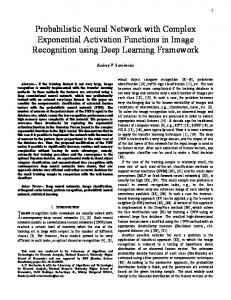
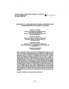
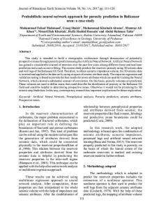
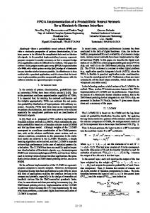
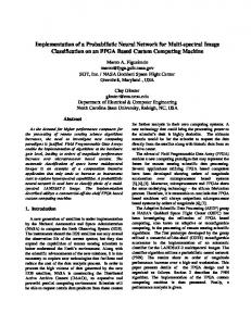
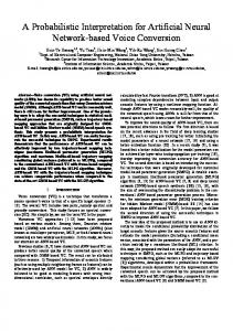
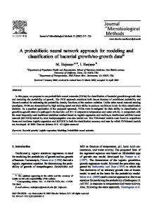
variability. Hence, diagnose such PD patterns, the ideology of classification of defects as suggested by CIGRE Working Group 21.03 [10] has been adopted. 1.1. PD Data acquisition and feature extraction PD is a complex random process. In order to obtain meaningful data for pattern recognition, it is necessary to acquire the fingerprints of the PD signals under well-defined conditions for which the cause of PD is known. For many years, PD recognition was performed by visual examination, i.e. on an oscilloscope screen. In recent years, the use of computeraided processing technique has facilitated the automation of the recognition task. As a result, the PD pulses are grouped by their phase angle with respect to 50 Hz (or 60 Hz) sine wave. Consequently, the voltage cycles are divided into phase windows representing the phase angle axis (0 to 360°). If the observation takes place for several voltage cycles, the statistical distribution of individual PD events can be determined in each window. By taking appropriate averages of these statistical distributions, the observed PD patterns throughout the whole phase angle axis result in two or three-dimensional patterns. A two-dimensional PD distribution Φ – q represents the PD magnitude apparent charge (q) as a function of phase angle (Φ) while a three-dimensional Φ – n – q represents the relationship between the PD magnitude ‘q’ and the pulse count ‘n’ as a function of phase angle. Each discharge pulse in the pattern reflects the physical process at the discharge site and a strong relationship has been found between the features of these patterns and the type of defect causing them. The method is independent of the electrical circuit between the defect and the detector. As long as the detection circuit reveals the phase angle and the relative phase height of the impulses it does not matter whether a discharge signal comes from complicated transformer windings or from a simple capacitor; the characteristics Φ – q is of interest. In order to ascertain the rationale behind the technique an investigation on the PD data is carried out using a PD meter (W.S. Test Systems Make, Type DTM-D), which has a frequency band of 1 MHz, with a built-in oscilloscope to display the PD pattern. Also ‘PD gold’ software (developed by HV Solutions Inc, UK) in a tablet PC is interfaced with the PD meter for displaying PD patterns in elliptical or on sinusoidal form. The software captures PD signals synchronously across 50 Hz (or 60 Hz) power cycle allowing the user to observe familiar phase-related patterns of discharge, online and in real time. The software provides an automatic PD threshold level for recording the number of pulses per power cycle. It also includes an automatic RF noise-reduction function, which uses single-frequency spectral subtraction. It also displays graphically the relation between Φ – q, q – n and time vs PD magnitude, respectively (Figs 1 and 2). For the purpose of recognition and classification, three PD sources of known fault have been fabricated. The internal discharge was generated by a void of dimension 1 mm diameter and 1.5 mm depth on a 12 mm-thick Perspex material of diameter 80 mm (Fig. 3(a)). The corona discharge (external discharge) was generated by an electrode of apex angle 85° attached to the HV bus (Fig. 3(b)). The corona discharge in oil (internal discharge) was generated with a sharp point immersed in transformer oil (Fig. 3(c)). The experimental setup, the discharge detector and software interfaced tablet PC are shown in Fig. 4.
282
B. KARTHIKEYAN et al.
(a)
(b)
FIG. 1. Relation between (a) Φ – q (void) and (b) q – n (void).
In this specific case, it has been found that for the discharge sources listed in Table I, time duration of 5 min is sufficiently long to capture the inherent characteristics of PD. It is very difficult to identify the input feature vector of the PD pattern for which the networks will respond better to a particular pattern of input. It is found in practice that the magnitude of discharge pulse (q), the number of discharge pulses (n) and the phase angle (ϕ) at which the discharge occurs are the three basic and major parameters used for pattern recognition. The numbers of fingerprints in the database were 55, of which 21 were patterns of defect type ‘A’, 17 of defect type ‘B’, and 17 of defect type ‘C’. The database and the corresponding applied voltage are shown in Table I. PO data for Channel 1
Time (minutes) FIG. 2. Time vs cumulative PD for an internal discharge (void).
A HEURISTIC COMPLEX PROBABILISTIC NEURAL NETWORK SYSTEM
283
(a)
(b)
(c)
Fig. 3. Fabricated PPD sources: (a): an electrode bounded void of size 1 mm diameter and 1.5 mm depth on 12 mmthick Perspex dielectric material; (b): a sharp edge of apex angle 85° for obtaining discharge patterns (external discharge); (c): a sharp edge of apex angle 85° in oil for obtaining discharge patterns (internal discharge).
Tablet Pc
PD meter Test Specimen (a)
Test Transformer
Coupling capacitor
(b) FIG. 4. (a) Experimental set-up and (b) discharge detector, tablet PC with PD analyzer.
284
B. KARTHIKEYAN et al.
Table I Applied voltage for PD fingerprints Defect type
Description
Applied voltage (kV)
Number of patterns
Total number of patterns
A
Electrode-bounded cavity at the HV electrode (Fig. 3(a)) Point-to-dielectric gap in air (Fig. 3(b))
C
Point-to-dielectric gap in oil (Fig. 3(c))
5 5 5 6 6 5 6 5 5 7
55
B
7.28 9.1 9.555 10.01 13.65 20.93 22.75 20.93 29.12 31.85
1.2. Knowledge-based feature extraction Classification of PD is based on recognition. There are two basic possibilities for recognizing discharges: phase- and time-resolved recognition. Time-resolved recognition has attractive advantages, since a direct relationship between the physics in the defect and the shape of the signal can be established and stages in the aging of the dielectric materials can be recognized. However, phase-resolved recognition is used in this approach for pattern recognition and classification since each discharge pulse in the pattern reflects the physical process at the discharge site and a strong relationship has been found between the characteristics of these patterns and the type of the defect causing them. Phase-resolved PD patterns (PRPD) are discharge patterns in relation to AC cycle [8]. The ϕ – q – n data assimilated with the assistance of computer-aided PD measurement and acquisition system is provided to the ANN black box as input in a suitable and compact form, which captures the attributes that correlate with the discharges. The compact form of representing the input data is called the preprocessed input and serves as fingerprints and forms the basis for classification. Many forms of features are extracted from the same PRPD pattern so as to identify the apt input characteristics vector for which the network responses well. The presence of a large number of input variables can present problems commonly referred to as the ‘curse of dimensionality’ in the pattern recognition task. One simple technique to help alleviate such problems is to combine input variables together in knowledge-based way to make a smaller number of new variables called ‘features’. These might be formed based on the understanding of the particular problem to be tackled. Various features are extracted from the deduced quantities based on measures of maximum and minimum values. Since PD phenomena that occur in dielectric media are inherently complex stochastic processes that exhibit significant statistical variability in properties such as pulse amplitude, shape and time of occurrence, the PD distribution is analyzed on two aspects, one it is viewed as discrete random process and on the other as continuous random process. Hence the statistical and stochastic measures have been introduced.
A HEURISTIC COMPLEX PROBABILISTIC NEURAL NETWORK SYSTEM
285
Various forms of fingerprints are: 1. Measures of maximum and minimum values from the PRPD patterns (a) (b) (c) (d) (e) (f) (g) (h) (i) (j)
Φ – qmax – n (phase window of 10° phase window width) Φ – qmin – n (phase window of 30° phase window width) ϕ – q – nmax (phase window of 10° phase window width) ϕ – q – nmin (phase window of 30° phase window width) Φ – qmax – n/Φ – qmin-n (phase window of 10° phase window width) Φ – qmax – n/Φ – qmin-n (phase window of 30° phase window width) ϕ – q – n (phase window of 360° phase window width) ϕ – q (phase window of 360° phase window width) Time vs PD (phase window of 360° phase window width) Time vs PD (phase window of 18° phase window width)
This method is simple and straightforward and involves using maximum/minimum values of q or n in each phase window as input to the NN. The phase angle of 10° and 30° is considered here so as to study the network response with small and large vector length. For instance, the Φ – qmax – n characteristic vector comprises an input length of 108 units for 10° (i.e. 3 characteristic parameters for each phase window width of 10°) and 36 units for 30° phase window width. 2. Measures of central tendency (values of q, n) (a) Mean, median and mode-phase window of 10 width (b) Mean, median and mode-phase window of 30° width 3. Measures of dispersion (values of q, n) (a) Range, mean deviation, standard deviation and quartile deviation–phase window of 10° width. (b) Range, mean deviation, standard deviation and quartile deviation–phase window of 30° width. Preprocessing ensures compactness and thus reduces the number of components of input to the NN. Also the efficacy of input is analyzed by providing the network with both reduced component vector and the entire data from the full window. The original probabilistic neural network is trained and tested for the aforesaid input vectors. 2. Pattern recognition and classification using neural networks The complexity of analyzing such PD patterns obtained from digital computer acquisition system is evident as this is a complex nonlinear problem. The process being stochastic the associated effects of memory propagation with the influence of residues from the previous PD pulses, etc. has made the classification of such PD patterns in terms of ϕ – q – n even more complex. Pattern recognition basically involves the identification of similar data within a collection, which resembles the new input. Since ANN has the ability to learn from examples, generalize well from training, handle noisy data conveniently, create its own re-
286
B. KARTHIKEYAN et al.
lationship amongst information and hence no equations, it has become an innovative technique suitable for PD pattern recognition and classification. Several types of ANNs have been used till date for the classification of PD patterns [1– 7]. However, a novel approach of using PNN [11–15] has been used for the classification of PD patterns for the following reasons: n n n n n n n
n n n n n
Training is minimal and instantaneous. Good generalization capability. It is easy to use and is extremely fast for moderate-sized data bases. Can be used in real time because as soon as one pattern representing each category has been obtained, the network can begin to generalize new patterns. On comparing the popular back propagation network (BPN) with the PNN it is observed that PNN trains faster than the BPN. The generalization accuracy is almost as good as and often better than that of BPN. The shape of the decision surface can be made as complex as necessary or as simple as desired by choosing an appropriate value of the smoothing parameter. However, this value influences the number of misclassifications. The decision surface can approach the optimal minimum risk decision surfaces. Erroneous samples and sparse samples are tolerated. An inherently parallel structure. Training samples can be added or removed without extensive retraining. No local minima issues as in BPN
2.1. Probabilistic neural network PNN was developed and formulated by Donald Specht [11], and is predominantly a classifier that maps input patterns to a number of classifications and can be utilized into a more general function approximator. It is a network formulation of ‘probability density estimation’ and is a model based on competitive learning with a ‘winner takes all attitude’ and the core concept based on multivariate probability estimation. It has no feedback path. It works on estimation of probability density function (pdf). The development of PNN relies on the Parzen window concept of multivariate probabilities. The Parzen window method is a nonparametric procedure that synthesizes an estimate of a pdf by superposition of a number of windows, replicas of a function. Its classifier takes a classification decision after calculating the pdf of each class using the training examples. The multicategory classifier decision is expressed as pk fk > pj fj, for all j = / = k where Pk is the prior probability of occurrence of examples from class k and fk is the estimated pdf of class k. The Parzen window classifier uses the entire training set of examples to perform classification, i.e. it requires storage of the training set in the computer memory. The speed of computation is proportional to the training set size. PNN is an implementation of a statistical algorithm called kernel discriminant analysis in which operations are organized into a multilayered feedforward network with four layers (Fig. 6): Input layer, pattern layer, summation layer and output layer. The input layer does not perform any operation and simply distributes the input to the exemplar layer. On receiving a pattern x from the input layer, the neuron Φij of the pattern layer computes its output
A HEURISTIC COMPLEX PROBABILISTIC NEURAL NETWORK SYSTEM
Input Layer
Layer Exemplar Pattern (or) Layer
Class/Summation Layer Decision Layer
287
Output Layer
FIG. 5. Architecture of probabilistic neural network.
Φij(x) = exp[(XTWki – 1)/σ2], where σ is the smoothing parameter, x, the input neuron vector, and W, the weight vector. The summation layer neurons compute the maximum likelihood of pattern x being classified into Ci by summarizing and averaging the output of all the neurons that belong to the same class NK
∑ exp[( xT wki − 1/ σ 2 ], i =1
where N is the number of examples and K, the number of classes. If the a priori probabilities for each class are the same, and the losses associated with making an incorrect decision for each class are the same, the decision layer unit classifies pattern x in accordance with the Baye’s decision rule based on the output of all summation layer neurons C(x) = arg(max{pi(x)}), i = 1, 2, …, m, where C(x) denotes the estimated class of the pattern x and m the total number of classes in the training samples. One outstanding issue in PNN is structure determination of the network, i.e. an appropriate smoothing parameter. 2.2. Significance of smoothing parameter The only parameter that has to be selected during training is the smoothing parameter σ. The role of the smoothing parameter on PNN is summarized after a detailed analysis. The important observations are as follows:
288
B. KARTHIKEYAN et al.
1. The recognition significantly depends on the value of sigma σ, which is selected on a trial-and-error basis. 2. The optimum value of smoothing parameter is obtained after conducting a detailed analysis and hence is time consuming. 3. In the actual case of training and testing, it has been observed that small changes in the value of the smoothing parameter do not change the misclassifications dramatically. 4. A quite obvious yet an important observation indicated is that a decrease in the value of the smoothing parameter led to the formation of the required decision surface, while at higher values over the actual responsive range insignificant changes were observed in the classification of the input of the network. 5. On detailed investigation it is inferred that the optimum value of sigma differs for each input vector type and also varies with respect to the length of the input (dimensionality). During the investigation it is observed that the recognition is optimum only for a particular value of sigma for any type of input. After a detailed analysis, it is observed that the smoothing parameter plays a vital role in classification and hence it is deciphered that the training pattern itself should take into account the optimum value of smoothing parameter. 2.3. Selecting the smoothing parameter on conditional grounds Generally the smoothing parameter is set to a value on trail-and-error basis. But an appropriate smoothing parameter is often data dependent. Therefore, it requires a proper procedure for the selection of smoothing parameter. A few studies [11] expound a way of finding the optimal value of sigma using genetic algorithm. When a neural-network classifier is constructed, classification accuracy and network size are the most important factors that need to be taken into consideration. The proposed flowchart runs in an iterative manner till the optimal value of σ is found. It is observed during investigations that the value of σ for which the summation layer produces an output other than zero for all classes is almost optimum. Here initially a smoothing parameter is randomly assumed as a small positive number. Further the algorithm of original PNN is altered in such a manner that an automatic adjustment to the parameter is made appropriately using the training patterns and the classification categories of the training patterns themselves. The modified flowchart of OPNN is shown in Fig. 6. 3. Discrimination of PD patterns using PNN The PNN paradigm has been evaluated experimentally for its ability to recognize the discharge pulse patterns associated with different discharge patterns. The number of discharge patterns, the applied voltage and their sources are shown in Table I. Various forms of inputs have been applied as features or attributes of the pattern form to the NN model to perform PD recognition. Initially the PNN is trained with nine patterns. The recognition task is first attempted with nine randomly selected patterns for training. The remaining patterns including the training exemplars are tested and observations are tabulated (Table II). The recognition is
A HEURISTIC COMPLEX PROBABILISTIC NEURAL NETWORK SYSTEM
289
FIG. 6. Flowchart of modified PNN. CR–Classification rate (ratio of training patterns correctly classified to the total training exemplars), θ: parameter (user defined), σ-smoothing parameter, σo: optimal sigma.
290
B. KARTHIKEYAN et al.
Table II Classification rate in percentage before and after hold-one-out validation Feature Feature identification type number 1 2 3 4 5 6 7 8 9 10 11 12 Discarded input types
Φ – qmax – n – 10° Φ – qmax – n – 30° Φ – q – nmax – 10° Φ – q – nmax – 30° Φ – qmax – n/Φ – qmin – n – 10° Φ – qmax – n/Φ – qmin – n – 30° Φ – qmax – n – 360° Φ – q – 360° Measures of central tendency–10° Measures of central tendency–30° Measures of dispersion–10° Measures of dispersion–30° Time vs PD – 360° Time vs PD – 18°
Nine training exemplars First set Second set BV AV BV AV
Twelve training exemplars First set Second test BV AV BV AV
78.18 92.72 60 61.81 69.09 89.09 61.81 61.8 80 87.27 80 92.72 43.6 49.1
87.27 94.55 83.63 76.36 80 92.72 80 80 81.8 89.09 85.45 96.36 40 49
84.31 100 64.7 66.66 74.51 96.08 66.66 66.66 86.27 94.11 86.27 100 – –
81.8 87.27 69.09 61.81 80 72.72 67.27 69.09 76.36 89.09 85.45 89.09 40 49
88.23 94.11 74.5 66.66 86.27 78.43 72.55 74.5 83.25 94.11 90.19 96.08 – –
94.12 100 90.19 82.35 86.27 100 86.27 86.27 90.19 94.12 92.16 100 – –
87.27 90.90 90.90 76.36 85.45 78.18 76.36 76.36 76.36 92.73 89.09 92.73 47.27 58
94.12 96.08 98.04 80.39 92.15 84.31 82.35 82.35 84.31 98.04 92.16 96.08 – –
BV: Before validation; AV: After validation.
quite good, mostly for all types of input. The paradigm has again been tested for its ability by another nine randomly selected training exemplars. The classification rate was not consistent with different training sets of same sequence and hence the paradigm has been presented by another 12 randomly selected training exemplars of two sets as above. Their test results and recognition rate as a measure of percentage are tabulated in Table II. It can be well construed that with a few training exemplars of each class, the PNN can capture the inherent attribute of each class and can respond satisfactorily. The performance of the network is also analyzed with 12 training exemplars. It can be observed that with increase in the number of training exemplars, the recognition rate has increased for all types of input feature vector. It can be inferred that with increase in the number of training exemplars, the number of misclassifications can be brought down; however, there exists inconsistency in recognition rate for some types of input types on both sets of training exemplars. An attempt is made in the next section to bring down the number of misclassifications by validating the inputs. 3.1. Training and performance evaluation The performance of a network after training has been completed is to be evaluated. Several methods are adopted for the validation of the network and the input, viz. partial set training, hold-one-out Training, and pathology analysis. The hold-one-out and the partial set training method are being adopted to evaluate the same. 3.1.1. Hold-one-out training A technique used to measure the effectiveness of network training is called, appropriately enough, the hold-one-out technique.
A HEURISTIC COMPLEX PROBABILISTIC NEURAL NETWORK SYSTEM
classification rate in %
100
100
100
98
94
92
98 98 98 96 96 90
88
86
84 84 80
291
78 74 74
74 72 71 68
71
PS1 PS2
64 60 1
2
3
4
5
6
7
8
9 10 11 12
Inputs
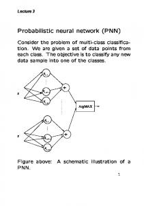
FIG. 7. Observations of partial set validation after removal of patterns found noisy using hold-one-out technique.
During the validation step adopted over the various forms of inputs, it is observed that a few patterns showed consistency in being misclassified. The patterns which showed inconsistency were identified and removed from the PD database and the training and testing procedure is repeated. Also the input feature vector involving time-resolved patterns (time vs PD) showed large number of misclassifications (Table II). These have been removed from the database of finger prints. It can be observed from Table II that the efficacy of recognition has greatly improved for all input vectors and for all sets of training patterns after validating the inputs. 3.1.2. Partial set training Apart from the hold-one-out technique, the effectiveness of the network is measured by presenting the network that is not a part of the training set. This is to evaluate how well the network can successfully learn from training exemplars. Among the 51 patterns, 27 have been used as training exemplars and the others including the training exemplars are tested. Similarly, the remaining 24 patterns are used as the second partial set and the above analysis is repeated. The observations are shown in Fig. 7. It is observed that the recognition rate is good in both the partial training set and is not even approximately the same for any type of input. Also, the partial set training methodology has inherent potential failings and can cause misleading interpretation of results. The common problem encountered is the sequence of the training set during network training. It is observed that there is inherent difficulty in identifying the exact training exemplars and the type of input vector for which the network will respond well. Hence a system needs to be developed which has a consistent recognition rate and is independent of the training exemplars set and the input vector. The problem is overcome by developing a composite network, which utilizes the benefit of all input features for good recognition rate. 4. Complex probabilistic neural networks It is observed from the analysis that each input feature vector has shown a few misclassifications; moreover, the misclassified patterns are not the same for all other types of input
292
B. KARTHIKEYAN et al.
FIG. 8. Architecture of composite probabilistic neural network system.
feature vector analyses for the same source data. It is also observed that the number of misclassifications depends upon the type and length of the input. Hence it is mandatory to design a complex system utilizing all forms of input vector at a time, so that the expected classification is of the highest order. This is accomplished with a simple composite network system shown in Fig. 8. In complex network system, one PD pattern is taken for classification. All types of input feature vector is extracted from the raw data in parallel. The input feature vectors are given to the corresponding networks. All the networks are trained by the same source of data. Output of all the networks is compared and frequently appearing class is taken as an output. A composite neural network system was designed and tested. It is clear from Table III that the CNN system has shown consistency in recognition rate for all the number of training exemplars and with any training set. So a deterministic decision can be made with CNN and necessary action can be taken on the insulation system offering PD. Table III Recognition rate with composite neural network Sets
First Second
Observations with Nine training exemplars
Twelve training exemplars
Partial set of training exemplars
86.27 88.23
92.15 94.11
100 96.16
A HEURISTIC COMPLEX PROBABILISTIC NEURAL NETWORK SYSTEM
5.
293
Conclusions
Several important conclusions have been deduced. They are: 1. The heuristic approach of finding the optimum value of smoothing parameter has reduced greatly the time for determining the optimum value manually and has obviated the need of an expert in the area of PNN. Also it is observed that the value of sigma found by trial-and-error basis almost matches with the automated value. 2. It is observed that the measures based on statistical operators responds better than the measures based on maximum and minimum values. 3. Validation using hold-one-out approach helps in resolving inconsistency in the inputs and assists in eliminating incompatible patterns. 4. The recognition rate is increased in partial set validation after removal of the mismatched patterns. 5. The complex neural network system involves all forms of inputs and enables in providing a deterministic decision about the class to which a defect belongs to. 6. This study can be extended to complex OPNN involving various kernel functions such as rotated kernel function, elliptical basis kernel function which may result in better recognition rate (The current work on CPNN adopts Gaussian kernel function). 7. Multidefect-type PD pattern classification and rejection of noise have not been taken up since the emphasis of the paper is primarily on ascertaining the ability and effectiveness of the proposed complex neural network to classify complex nonlinearity involved in PD patterns. 8. The analysis undertaken in this OPNN can also be studied on other versions of PNN, which may yield better recognition rate. Also, a hybrid network comprising various complex networks on PNN can be developed for validation on one type of PNN with other variations of the same kind. 9. The development of this technique has now reached a stage that needs some more experience on the actual use of system. Improvements might be obtained by trying out this complex technique with a few alternative neural networks meant for the classification task. References 1. C. Cachin, and H. J. Wiesman, PD recognition with knowledge based preprocessing and neural networks, IEEE Trans. Dielectr. Electr. Insul., 2, 578–589 (1995). 2. R. Candela, G. Mirelli, and R. Schifani, PD recognition by means of statistical and fractal parameters and a neural network, IEEE Trans Dielect. Electr. Insul., 7, 87–94 (2000). 3. E. Gulski, and F. H. Kreuger, Computer aided recognition of partial discharges, IEEE Trans. Electr. Insul., 27, 82–92 (1992). 4. E. Gulski, and A. Krivda, Neural network as a tool for recognition of partial discharges, IEEE Trans. Electr. Insul., 28, 984–1001 (1993). 5. Hans-Gerd Kranz, Diagnosis of partial discharge signals using neural networks and minimum distance classification, IEEE Trans. Electr. Insul., 28, 1016–1024 (1993).
294
B. KARTHIKEYAN et al.
6. T. Hong, M. T. C. Fang, and D. Hilder, PD classification by a modular network based on task decomposition, IEEE Trans. Dielectr. Electr. Insul., 3, 207–212 (1996). 7. M. Hoof, B. Friesekben, and R. Patsch, PD source identification with novel discharge parameters using counterpropagation neural networks, IEEE Trans. Dielectr. Electr. Insul., 4, 17–32 (1997). 8. F. H. Kreuger, E. Gulski, and A. Krivda, Classification of partial discharges, IEEE Trans. Electr. Insul., 28, 917–939 (1993). 9. K. Z. Mao, K. C. Tan, and W. Ser, Probabilistic neural network structure determination for pattern classification, IEEE Trans. Neural Networks, 11, 1009–1016 (2004). 10. IEC, 60270–1999, Partial discharge measurements. 11. Working Group 21.03, CIGRE Recognition of discharges, Electra, 11, 61–98 (1969). 12. Donald F. Specht, Probabilistic neural networks for classification, mapping or associative memory, Proc. IEEE Int. Conf. Neural Networks, Vol. 1, 525–532 (1988). 13. Donald F. Specht, and Philip D. Shapiro, Generalization accuracy of probabilistic neural networks compared with back-propagation networks, Proc. Int. J. Conf. on Neural Networks, Vol. 1, pp. 887–892, Seattle, WA, July 1991. 14. T. P. Washburne, Donald F. Specht, and R. M. Drake, Identification of unknown categories with probabilistic neural networks, Proc. IEEE Int. Conf. Neural Networks, Vol. 1, pp. 434–427, San Francisco, March 28– April 1, 1993. 15. D. F. Specht, and H. Romsdahl, Experience with adaptive probabilistic neural network and adaptive general regression neural network, Proc. IEEE Int. Conf. Neural Networks, Vol. 2, pp. 1203–1208, Orlando, FL, June 28–July 2, 1994. 16. Donald F. Specht, Probabilistic neural network and the polynomial adaline as complementary techniques for classification, IEEE Trans. Neural Networks, 1, 111–121 (1990).