A hybrid approach to predict residual stresses induced ... - LMT Cachan

A hybrid approach to predict residual stresses induced by ball-end tool finishing milling of a bainitic steel Nicolas GUILLEMOT1,2,a, Benoît BEAUBIER2,b , Tarek BRAHAM3,c , Claire LARTIGUE1,a, René BILLARDON2,b 1

LURPA, ENS-Cachan, Université Paris-Sud 11,

2

LMT-Cachan, ENS-Cachan / CNRS (UMR 8535) / UPMC (Paris 6) 61, avenue du Président Wilson, 94235 Cachan Cedex, France

3

LAMPA, Arts et Métiers Angers, 2, boulevard du Ronceray, 49100 Angers, France

a

[email protected], [email protected], [email protected], d e [email protected], [email protected]

Keywords: Ball-end finishing milling, tool inclination, oblique cutting, Infra-Red camera measurements, numerical simulation.

Abstract. The objective of this study is to predict the residual stresses induced by ball-end milling using an hybrid approach based on a numerical simulation where thermo-mechanical loads equivalent to the cutting process are applied directly on to the final surface of the workpiece without modelling the material removal. The applied loading is derived from the measurement of the maximum cutting forces and the measurement by IR camera of the temperature in the tertiary shear zone. The 2D simplified model proposed herein is derived from the analysis of oblique cutting with elementary cutting tools and makes it possible to take account of the normal rake and local helix angles as well as the lead angle of the tool. The feasibility of the approach is assessed by comparing experimental measurements and numerical predictions of the residual stresses induced by ball-end tool finishing milling of flat specimens made of a bainitic steel. Introduction The accuracy of the prediction of the behaviour of machined parts, in particular their fatigue life, is dependent on the knowledge of their initial mechanical state, including the residual stresses induced by the machining process. Conversely, a reliable prediction of the residual stresses induced by the machining process could be used to optimize this process in order to improve the fatigue life of the workpiece. For instance, the machining strategy –viz. tool inclination and cutting parametersduring finishing ball-end tool milling could be controlled in order to induce compressive residual stresses in the subsurface of the workpiece – which have a positive influence on its fatigue life. Three main different approaches can be used to predict the residual stresses induced by machining. Analytical approaches can be revisited. For instance (see [1]), it has been recently proposed to use Oxley energy partition model [2] to derive the thermal flow in the Primary Shear Zone (PSZ). This temperature field is then used as an input for a thermo-mechanical calculation carried out to determine the stresses applied to the workpiece. The residual stress profile in the depth beneath the machined surface is finally determined after material removal. Computation time is very small – typically a few seconds- but the description of the cutting phenomenon is not representative of the real process since the partition of the forces between the different Shear Zones (SZ) is not taken into account. Most recent studies in this field are related to the development of numerical simulations of material cutting and removal – using, in most cases, various forms of the finite element method. So far, this approach has been mainly applied to orthogonal turning process [3-4]. The limitations of this approach are high computation costs, and dependence of the results on friction and material

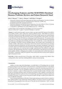
constitutive models – which are very difficult to assess within the range of thermo-mechanical loading induced by the cutting process. Typical duration of a simulation is about 10 days when this approach is applied to milling [5]. The hybrid approach consists in a simplified numerical approach where thermo-mechanical loads equivalent to the cutting process are applied directly on to the final surface of the part (Fig. 1 right) without modelling the material removal itself [6]. Residual stresses are generated after thermomechanical loading and stress relaxation. These loads in the Primary and Tertiary Shear Zones (PSZ and TSZ) are derived from cutting force and temperature measurements. Recently proposed and applied to turning, this approach leads to results with a good correlation with results of complete standard numerical simulations although computation costs are significantly reduced [6]. The final objective of this study is to develop and apply to ball-end milling the hybrid approach first proposed and applied to turning by Valiorgue et al. [6]. To first prove the feasibility of the approach, the results presented in this paper are restricted to a 2D model. Fig. 1 summarizes the main steps of the hybrid approach applied to ball end-tool milling process. Constitutive law of the material

Cutting forces Mesure d’efforts measurement Chargement Mechanical mécanique loading

Cutting conditions Thermal loading

p’ q’

Z Y

Thermo-mechanical loading

Finite elements analysis

- Distribution of forces in the ZCT

- Loading interval: radial depth of cut

- Spatial distribution of the loads

-2D simplification

Temperatures measurement by IR thermography

ae

ae

Residual stresses

Overview of the hybrid modelling for milling

Fig. 1: Hybrid approach for milling process. Mechanical loads equivalent to the cutting process are derived from the measurement of global cutting forces. Specific difficulties induced by ball-end tool milling are due to the fact that cutting is not orthogonal and that the inclination of the tool relative to the surface may vary. Therefore, it is proposed to divide the tool into elements – or Elementary Cutting Tools (ECT). Using the oblique cutting approach [7] and taking account of the tool-surface inclination [8-9], the local cutting forces are determined on each (ECT) and on the TSZ. Then, the real load p’ applied on to the final surface after removal of the chip is computed (Fig. 1). The thermal flux q’ associated to the mechanical load is derived from an inverse analysis based on the comparison between the maximum value of the temperature used in the numerical simulation and the temperature measured with an Infra-Red camera. Finally, the thermo-mechanical loading is moved on to the final surface in order to simulate the successive cutting passes. The distance between each loading corresponds to radial depth of cut, ae. In the following, the approach is presented in details and applied to the prediction of the residual stresses in a flat workpiece made of a bainitic 25MnCrSiVB6 steel. DESCRIPTION OF THE APPROACH A model to derive mechanical loading from cutting forces measurements Finishing milling process with a ball-end tool. Parameters used in ball-end tool finishing milling are defined on Fig. 2. During milling, the tool lets furrows the height of which, called cusp height, is linked to radial depth of cut, ae, and tool radius, R. The movement of the tool is characterized by cutting speed, Vc, and feed per tooth, fz, which are respectively controlled through spindle frequency, N, and feed rate (in the machining direction), Vf. The inclination of the tool with respect to the normal to the surface –in the plane containing this normal and the feed rate- is characterized by lead angle, βf. The cutting process can be locally analyzed in the 3D elementary zone (3DEZ).

200

θ1

N

Fx

θ2 θ3 θ4 θ5

Fy 100

Cutting forces (N)

r n 3DEZ ae

βf

Vf

hc

Fz

0 0

90

180

270

360

450

-100

-200

Z

-300

X

Entry of the second tooth in the material

Entry of the first tooth in th material

Y

-400

Rotation angle of the tool (°)

Fig. 2: Milling parameters

Fig. 3: Cutting forces measurement.

Cutting forces measurements. Results reported in Fig. 3 derive from measurements performed with a KISTLER 9443 triaxial force dynamometer for machining conditions defined in the application paragraph. The extreme value of all cutting force components correspond to the same value, θ4, of the rotation angle. This value is defined relatively to angle, θ1, corresponding to the entry of the tool in the material (Fig. 3). For this value of the rotation angle, identified as θ4 = 160°, cutting force component Fy is positive. Value, θ4, of rotation angle, and cutting force components, Fx, Fy and Fz, are the entries of the model developed to derive the mechanical loading equivalent to the cutting process. Elementary forces in the shearing zones. The geometry of the ball-end tool is defined in Fig. 4. The cutter contact is located by tool rotation angle, θ, and angle χ between the Z-axis and the cutter point of the flute. The spherical reference frame (er, eθ, eχ) is used to define elementary cutting forces dFr, dFt and dFa (respectively radial, tangential and axial) applied to the workpiece.

Q-Q R(Z)

Q Z

Y χ

dZ

X

dFc

θ

tn e θ db

γn

Z

eχ er

Q

Y

dFc1

eχ

eθ

er

dFr

dFr1 dFc2

X Vf

Tool

dFr2

Fig. 4: Geometry of the ball-end tool.

Fig. 5: Force assessment on the tool.

Valiorgue et al. assume that the final workpiece after removal of the chip is only subjected to stresses in the (TSZ) [6]. Fig. 5, which corresponds to a cut along Q-Q as defined in Fig. 4, shows one tooth with a normal rake angle, γn. Subscripts 1 and 2 of cutting force components refer to the SSZ and TSZ, respectively. Cutting and radial components dFc and dFr on the tool are given by

dFc = dFr1 sin γ n + dFc1 cos γ n + dFc 2  dFr = −dFc1 sin γ n + dFr1 cos γ n + dFr 2

dFc1 ⋅ µ1 = dFr1 where  dFc 2 = dFr 2 ⋅ µ 2

(1)

For oblique cutting, the cutting components should be decomposed so that

dFa1 = dFc1 sin i dFt1 = dFc1 cos i and  (2)  dFa 2 = dFc 2 sin i dFt 2 = dFc 2 cos i where dFa and dFt are the axial and tangential components. The elementary radial cutting component in the TSZ can be expressed from resultant elementary forces so that dFc (µ1cγ n − sγ n ) − dFr (µ1 sγ n + cγ n ) (3) µ 2 (µ 1 c γ n − s γ n ) − µ 1 s γ n − c γ n The aim of the following oblique cutting modelling is to determine dFr2 and then components dFa2 and dFt2 using Eq. 1 and 2. dFr 2 =

Modelling oblique cutting. To predict cutting forces for helical ball-end tools, Armarego [10] as well as Lee and Altintas [7] assume that the tool geometry can be represented by elementary cutting segments for which oblique cutting is considered. The spherical components derived from the model proposed by Armarego [10] are such that  dFr = K rc ⋅ Ad e + K re .dS   dFt = K tc ⋅ Ad e + K te .dS dF = K ⋅ Ad + K .dS ac e ae  a

(4)

where (Krc, Ktc and Kac) and (Kre, Kte and Kae) respectively denote the sets of cutting force and edge force coefficients, which are constant and unknown. Parameters Ads and dS respectively denote the elementary section of the chip and the length of a curved cutting edge segment. Area Ads, depending on uncut chip thickness, tn, and elementary width, db, may also be expressed as a function of the feed per tooth and elementary height of the uncut chip so that

dZ ⋅ f z sin θ sin χ = f z sin θ ⋅ dZ (5) sin χ According to Merchant theory [11] for orthogonal cutting, tangential and radial forces can be derived from shear angle, φn, normal rake angle, γn, normal friction angle, βn, and shear stress, τs. Ad e = db ⋅ t n =

Rake face

η ≈i Chip

dFc

dFa i

i

dFt dFr

db tn

Element of the cutting edge

Relief face

Primary shear zone

Fig. 6: Elementary forces in oblique cutting. For oblique cutting with an acute angle i (Fig. 6), coefficients Krc, Ktc, Kac can be calculated using the Armarego transformation [10]. Furthermore, Stabler rule [12], where parameter η is chosen equal to i, allows the simplification of the expressions so that

τs sin( β n − γ n )   K rc = sin(φ ) cos(i ) c n  τ s cos( β n − γ n ) + tan 2 i ⋅ sin β n   K tc = sin(φ n ) c   τ s [cos( β n − γ n ) − sin( β n )] tan i  K ac =  sin(φ n ) c

with

c = cos 2 (φ n + β n − γ n ) + tan 2 i ⋅ sin 2 β n

(6)

In [7], the cutting and edge coefficients are identified from orthogonal cutting tests for several feed and cutting speed values. As demonstrated in [10], Kae is generally negligible. The approach developed in this study to determine the cutting force coefficients (6) relies on orthogonal cutting tests considering a value of the feed per tooth used for milling. Cutting forces, Fr, Ft, and shear angle, φn, (through the deformed chip thickness [7]) are investigated for different values of cutting speed, representative of effective cutting speed Veff along the cutting edge. R( Z ) (7) Vc = Vc sin χ R0 Shear and friction angles are derived from orthogonal cutting forces, local normal rake angle, γn, feed rate, f, and chip thickness, tc, with the following expressions Veff ( Z ) =

F  f cos(γ n )   (8) ; β n = γ n + tan −1  r   t c − f sin(γ n )   Ft  For each cutting speed during orthogonal cutting tests, the shear stress is given by 

φ n = tan −1 

Ft + Fr cos(φ n + β a − γ n ) 2

τ s (Z ) =

(9)

2

(10) w ⋅ f / sin φ n where w denotes the wide of cut in orthogonal turning. For ball-end tool application [8], the acute angle i corresponds to the local helix angle and is given by

 R( Z )  i ( Z ) = tan −1  tan i0 sin χ  (11)  R0  where R0 and R(Z) denote the tool radius and the effective radius, respectively. For a finishing axial depth of cut equal to 0.5 mm, the local helix angle i(Z) is small so that length dS can be approximated by the width of the chip, db. Influence of the tool inclination. The influence of the tool inclination is taken into account through the measured resultant forces. Nevertheless, the local helix angle i(Z) plays a major role on the distribution of elementary forces (Fig. 6). Indeed, the helix angle varies from 0° at the end of the tool to i0 in the cylindrical area.

βf (a)

χ

χ

βf

(b) Fig. 7: Positive (a) and negative (b) lead angle of the tool.

Introducing a positive or a negative lead angle of the tool (see Fig. 7), the previous expression of this angle becomes:

 R( Z )  (12) i ( Z ) = tan −1  tan i0 sin (χ + β f )  R0  Finally, on each segment, the calculation of the cutting force coefficients relies on the effective cutting speed and on orthogonal cutting tests for a specific feed per-tooth. Determination of the edge force coefficients. The edge force coefficients, which are assumed to be constant all along the edge, are obtained from the measurement of resultant cutting forces, Fx, Fy and Fz in the Cartesian coordinate system  a p dF   Fx (θ )   ∫z = 0 x   F (θ )  =  a p dF   y   ∫z =0 y   Fz (θ )   a p dF   ∫z = 0 z  The elementary forces in the Cartesian coordinate system are obtained by:

(13)

 dFx (θ )   sθ ⋅ sχ cθ sθ ⋅ cχ   dFr  dF (θ ) = cθ ⋅ sχ − sθ cθ ⋅ cχ   dF  (14)  y    t   dFz (θ )   − cχ 0 sχ  dFa  with cθ = cosθ and sθ = sinθ. Elementary cutting forces, dFr, dFt and dFa, are added along the cutting edge and substituted by the Eq. 4, 5 and 6. Edge force coefficients are derived from resultant cutting forces measurement and Eq. 4.

2D representation od a 3D movement Contrary to turning, in milling, the chip thickness and thus the mechanical loads vary during the rotation of the tool. One rotation of the tool can be simulated in the 3D elementary zone (3DEZ) illustrated in Fig. 2. However, since small forces lead to low temperatures, it can be assumed that residual stresses are essentially due to maximum forces and maximum temperatures. Therefore, it is proposed herein to simulate the 3D cutting phenomenon by a 2D model of the elementary zone (2DEZ) corresponding to angle θ4 for which cutting forces are extremum. As seen in Fig. 8 and 3, for a small cusp height (5 µm), θ4 is close to π. To simplify, residual stress σyy induced by successive passes (with a radial depth of cut, ae) can be obtained by repeating thermo-mechanical loads in the 2DEZ for θ = π. N ae

Y θ4 2DEZ

X

Fig. 8: 2DEZ where cutting forces are maximal.

Fig. 9: Contact area measurement in the TSZ.

A hybrid modelling is thus used in the 2DEZ in the Y direction. To summarize, the procedure to derive the mechanical loading consists in 5 main steps: 1. Computation of the spherical cutting forces components on each segment of the cutting edge from orthogonal cutting tests and resultant forces Fx, Fy and Fz. 2. Computation of elementary forces, dFr2 and dFa2, in the TSZ of each segment. 3. Measurement of the contact length in the TSZ, assimilated to the wear area (Fig. 9). The mean radial pressure, assimilated to a plane-cylinder contact is derived from Hertz theory as 2dFa 2 2dFr 2 (15) and dPa 2 = π a ⋅ db π a ⋅ db where a denotes the semi-length of the contact area as shown in Fig. 9. The last steps correspond to simulations allowing the transfer from the 2DEZ to the final 2D surface after material removal. 4. Identification of displacements Ux and Uz on the final milled surface. 5. Simulation of the mechanical load by these displacements to obtain the forces on the mesh elements and then the resulting pressure distribution (Fig. 10). dPr 2 =

Path n+1

Z

Path n

Y

ar dZ

ap

χ 2DEZ

db

Initial loading at the interface tool-part

Resulting loading applied on the final workpiece

Fig. 10: Transition from the mechanical loads on 2DEZ to loads subjected by the final surface.

Identification of the thermal flux density Heat generated by high plastic strains and friction is principally drained in the chip, in the tool, partially in the air and in the machined surface. Valiorgue et al. [6] proposes to derive the heat flux distribution from the mechanical power. Shi et al. [11] suppose that 85% of the cutting power is transformed into heat. Then, 10% of this flux is transferred to the work piece [12]. However, these partitions are very dependent on the tool and the material. More recently, Bonnet et al. [13] identify the partition of heat transfer in a TA6V part from mechanical power. The heat transfer coefficient in the part is an empirical formula derived from tribology measurements and depending on slip speed. In this study, with intermittent cutting, the heat flux is identified by simulation, comparing simulation results to temperatures evaluation with a CEDIP Jade III type Infra-Red camera. The measurement is carried out at a 1000 Hz frequency on a 64×128 pixels window. The available range of temperatures is 150-300°C. The contact area between surface and tool is represented in Fig. 11 (a). The temperature distribution, caused by friction of the relief face of the tool on the material, is uniform along the edge and the maximum temperature measured is 207°C. Unfortunately, the scanning frequency of the camera is too low to measure the heat flux and to ensure that the maximum temperature during the rotation of the tool is recorded. Hence, the numerical simulation is used to identify the heat flux. For simplicity sake, as a first approximation, the thermal flux density is taken constant in the cutting area, whereas the real flux is supposed to be dependent on local cutting forces. Considering Vc = 300 m/min and the cutting forces measurement, the time necessary to reach the maximum cutting forces is 0.35 10-3s. The heat flux density is applied during the same duration. This flux is obtained by inverse identification. The maximum temperature simulated on the surface is 208°C for a load of 115 W.mm-2.

Only the area affected by the temperature on the final surface, i.e. 0.6 mm after material removal (Fig. 11 (b)) for the application case, is simulated for the numerical.

0.5 mm

1.5 mm

Feed direction for βf = -3° 0.6 mm

Z Y

Area where the final surface is affected by thermal loading

1,5 mm

4.2 mm 1,92 mm

T°C max = 207°C

(a) Infra-Red thermography pictures

(b) Simulation of thermal loading on the 2DEZ

Fig. 11: Identification of maximum temperature and thermal flux density.

Numerical simulation In order to assess the residual stress profile down to 500 µm beneath the machined surface, the depth of the final 2DEZ is chosen equal to 1 mm. To allow for the simulation of several successive tool passes while avoiding side effects due to thermal reflection, the length of the final 2DEZ is also chosen long enough. Thermo-mechanical loads corresponding to the cutting edge paths tend to create plastic strain in the material. Then, residual stresses are obtained after stress unloading, i.e. equal to zero. The numerical simulation coupling thermal and mechanical effects is illustrated by the following case.

APPLICATION AND RESULTS Material behavior The workpiece material is a 25MnCrSiVB6 high-strength bainitic steel (marketed as METASCO MC). The elastoplastic behaviour of the material is modelled by a simple elastoplastic model with an Armstrong-Frederiks non linear kinematic hardening. Tensile experiments show that viscosity is negligible from 10-3 s-1 to 10-1 s-1 strain rate. As a first approximation, viscosity is assumed to be negligible even at 105 s-1 rate as this characteristic is inherent to the material. The values of Young's modulus, E, yield stress, σy, and hardening parameters, C1 and γ1, identified from tests under monotonic and cyclic loading, are given for room temperature and 200°C (Table 1). Thermal properties of the material, which are assumed to be constant in the range of values 20-200°C, are also given in Table 1. Table 1: Material parameters for simulation

20°C 200°C

Mechanical parameters E C1 σy [GPa] [MPa] [MPa] 190 565 157 190 510 52

γ1 767 346

Thermal parameters ρ C λ -3 -1 -1 [kg.m ] [J.K .kg ] [W.m-1.K-1] 7800 440 47 7800 440 47

α [K-1] 12.10-6 12.10-6

Machining conditions Cutting tests were performed with a 4-tooth ball-end tool with two teeth being for roughing. The tool is 10 mm in diameter with a helix angle of 30°. The workpiece was machined on a 5-axis MIKRON UCP710 milling centre. To be representative of finishing milling, ap is chosen equal to 0.5 mm. Cutting preliminary studies enabled to select cutting conditions generating maximum compressive residual stresses, viz. hc = 5 µm, Vc = 300 m/min, fz = 0.2 mm/tooth, and βf = -3°.

Residual stresses distribution Identification of the mechanical distribution. For the case considered (hc = 5 µm, Vc = 300 m/min, fz = 0.2mm/tooth, βf = -3°), cutting forces are maximal for θ4 = 160° and forces plots (Fig. 3) show that the real feed is 0.4 mm/tooth which is due to the fact that the two rough teeth (Fig. 9) do not participate to the cutting phenomenon for a low tool inclination and a depth of cut ap = 0.5 mm. The mean effective cutting speed Veff is less than 120 m/min (cf Eq. (7)) for an inclination βf = 3°. Moreover, orthogonal tests exhibit a constant shear angle of 65°. This angle is deduced from Eq. (8) and chip thickness measurement. These orthogonal tests also identify a constant friction coefficient µ = Fr/Ft = 0.58 between 50 and 200 m/min. The normal rake angle is constant and equal to 5° which leads to an angle βn = 35° (Eq. (9)). Shearing stress vary between 340 MPa near the axis of the tool to 180 MPa for Veff = 120 m/min. The values of the edge coefficients derived from forces given in Fig. 3 are given in Table 2. Table 2: Edge force coefficients Kre [N.mm-1]

Kte [N.mm-1]

Kae [N.mm-1]

48 35 0 Then, elementary forces, dFr2 dFt2 and dFa2, on each segment are calculated using (13-15). The friction coefficient of the secondary shear zone µ1 = 0.58 is derived from orthogonal cutting tests. Moreover it is assumed that µ1 = µ2 = 0.58. The elementary surface forces used in the simulation are obtained with Eq. 16 in which the parameter a = 35 µm is derived from Fig. 9.

Thermo-mechanical simulation. Fig. 12 displays the results of the simulation considering several successive passes in the Y direction. The thermal simulation induces a temperature field. Subsequently, the mechanical pressure dPr2 is imposed considering a thermo-elasto-plastic behaviour with non-linear hardening. Component dPt2 is not relevant in the plane Y-Z and dPa2 is considered as being almost null. Residual stresses σyy (MPa)

200

100

0 0

50

100

150

200

250

300

350

400

-100

-200

-300

115 W.mm-2 Expérimental

-400

-500

Depth beneath the machined surface (µm) Fig. 12: Residual stress distribution.

The stress field in the subsurface is heterogeneous and repetitive in the surface, which corresponds to the radial depth of cut. A residual stress profile is extracted from the result of the simulation (Fig. 1) and it is compared with the corresponding experimental result. In spite of a small offset, the evolutions of the two residual stress profiles are similar (Fig. 12). Predicted residual stresses are compressive within the range −260 MPa to −320 MPa in the close surface. Down to 30 µm beneath the machined surface, stresses tend to be less compressive as experimentally observed. Below 200 µm, both profiles slowly decrease towards 0 MPa.

CONCLUSION Despite the strong approximations made herein as well as the complexity of the thermo-mechanical loading induced by this cutting process, this study proves the feasibility of the hybrid approach to predict the residual stresses induced by ball-end milling – at least for cutting conditions inducing compressive residual stresses. The simplified model proposed herein leads to a 2D simulation considering that residual stresses are due to the maximal cutting forces and temperatures associated to a particular rotation angle. However, thanks to an oblique cutting analysis, the model takes into account the normal rake angle, the local helix angle of the tool as well as the tool inclination – via the lead angle. Inputs of the model are cutting force and temperature measurements. Furthermore, orthogonal cutting tests allow the identification of the shear stress, the friction and the shear angles, which all vary with the effective cutting speed. The edge coefficients are deduced from global cutting force measurements. The simulated residual stress field is obtained in the plane Y-Z by successive passes of the tool at a distance equal to the radial depth of cut. The results of this approach applied to finishing milling of a bainitic steel were favourably compared to experimental results. The approach should be applied to other cutting conditions to assess its predictive efficiency. Moreover, further work is required to extend the 2D model proposed herein to a 3D model which should allow for more realistic 3D results.

ACKNOWLEDGEMENTS The authors would like to thank gratefully ASCOMETAL CREAS for supplying material (25MnCrSiVB6, marketed as METASCO MC).

REFERENCES [1] D. Ulutan, B. Erdem Alaca, I. Lazoglu : Mater. Process. Tech. Vol. 183 (2007), p. 77-87. [2] P.L.B. Oxley: Mechanics of Machining: An Analytical Approach to Assessing Machinability, (Ellis Horwood Ltd., Chichester, England, 1989). [3] J.C. Outeiro, D. Umbrello, R. M’Saoubi : Inter. J. Mach. Tools Manufact. Vol. 46 (2006), p. 1786-1794. [4] J. Rech, H. Hamdi, S. Valette, in: Machining: Fundamentals and advances, edited by J. Paulo Davim, Chapter 3, Springer, (2008). [5] A. Maurel, M. Fontaine, S. Thibaud, G. Michel, J.C. Gelin: 11th Esaform conference on material forming (2008). [6] F. Valiorgue, J. Rech, H. Hamdi, P. Gilles, J.M. Bergheau: J. Mater. Process. Tech. Vol. 191 (2007), p. 270-273. [7] P. Lee, Y. Altintas: Inter. J. Mach. Tools Manufact. Vol. 9 (1996), p. 1059-1072. [8] M. Fontaine, A. Moufki, A. Devillez, D. Dudzinski: J. Mater. Process. Tech. Vol. 189 (2007), p. 73-84. [9] A. Lamikiz, L.N. Lopez de Lacalle, J.A. Sanchez, M.A. Salgado: Inter. J. Mach. Tools Manufact. Vol. 44 (2004), p. 1511-1526. [10] E.J.A Armarego, R.C. Whitfield: Ann. CIRP Vol. 34(2) (1985), p. 65-69. [11] G. Shi, X. Deng, C. Shet: Elsevier Sciences Vol. 43 (2002), p. 573-587. [12] A.O. Schmidt, R.J. Roubik : ASME 71 (1949), p. 245-252. [13] C. Bonnet, G. Poulachon, J. Rech, Y. Girard: Proceeding of the 12th CIRP Conference on Modeling of Machining Operations (2010), p.237-242.