A Hybrid Segmentation Method Applied to Color Images and 3D Information Rafael Murrieta-Cid1 and Ra´ ul Monroy2 1
2
Centro de Investigaci´ on en Matem´ aticas
[email protected] Tec de Monterrey, Campus Estado de M´exico
[email protected]
Abstract. This paper presents a hybrid segmentation algorithm, which provides a synthetic image description in terms of regions. This method has been used to segment images of outdoor scenes. We have applied our segmentation algorithm to color images and images encoding 3D information. 5 different color spaces were tested. The segmentation results obtained with each color space are compared.
1
Introduction
Image segmentation has been considered one of the most important processes in image analysis and pattern recognition. It consists in partitioning an image into a set of different regions such that each region is homogeneous under some criteria but the union of two adjacent regions are not. A poor segmentation method may incur in two types of errors: i) over-segmentation, meaning that an object is split into several different regions; and ii) under-segmentation (which is the worst), meaning that the frontier of a class is not detected. Existing segmentation approaches can be divided into four main categories: i) feature based segmentation (e.g. color clustering), ii) edge based segmentation (e.g. snake, edging), iii) region-based segmentation (e.g. region growing, splitting and merging) and iv) hybrid segmentation [7]. More recent methods in image segmentation are based on stochastic model approaches [1, 6], watershed region growing [17] and graph partitioning [19]. Some segmentation techniques have been especially developed for natural image segmentation (see for instance [2]). In this paper, we introduce a segmentation method, which provides a precise and concise description of an image in terms of regions. The method was designed to be a component of a vision system for an outdoor mobile robot. This vision system is capable of building a global representation of an outdoor environment. It makes use of both an unsupervised scene segmentation (based on either color or range information) and a supervised scene interpretation (based on both color and texture). Scene interpretation is used to extract landmarks and track them using a visual target tracking algorithm. This vision system has been presented in several various papers [8–11]. However, the segmentation method,
2
Murrieta-Cid and Monroy
about its main component, has never been reported on at an appropriate level of detail. In the design of our segmentation method, we were driven by the following assumption: unsupervised segmentation on its own without classification does not make any sense. This is because a region cannot be labelled without an interpretation mapping it to a known element or class. Thus, our segmentation method is designed to be embedded in a bigger system and satisfies the system specification. What counts as a correct segmentation has no universally accepted answer; some researchers argue the segmentation problem is not well-defined. Following a pragmatical perspective, we take a good segmentation to be simply one in which the regions obtained correspond to the objects in the scene. Our method rarely incurs in under-segmentation and, since it yields a small number of regions, has an acceptable over-segmentation rate. Given that our method produces regions that closely match the classes in a scene and that there tend to be a small number of regions, the computational effort required to characterize and identify a region is greatly reduced. Also, statistically speaking, the more accurate one region captures a class, the more representative the features computed out of it will be. 1.1
Related work
Feature thresholding is one of the most powerful methods for image segmentation. It has the advantage of small storage space and ease of manipulation. Feature thresholding has been largely studied during the last 3 decades [12, 14, 15, 18, 5]. Here, we describe briefly the most relevant work in the literature (for a nice survey, the reader is referred to [18].) In [12], Otsu introduced a segmentation method which determines the optimal separation of classes, using an statistical analysis that maximizes a measure of class separability. Otsu’s method remains as one of the most powerful thresholding techniques [18]. It was not until recently that we have seen enhancements to this algorithm [15, 5]. In [15], Liao et al. presented an algorithm for efficiently multilevel thresholding selection, that makes use of a modified variance of Otsu’s method. This algorithm is recursive and uses a look-up table so reducing the number of required operations. In [5], Huang et al. introduced a technique that combines Otsu’s method and spatial analysis. So, this technique is hybrid. The spatial analysis is based on the manipulation of a pyramid data structure with a window size adaptively selected according to Lorentz’s information measure. There also are thresholding techniques that do not aim at maximizing a measure of class separability, thus departing from Otsu’s approach [14, 22]. In [14], the authors presented a range based segmentation method for mobile robotics. Range segmentation is carried out by calculating a bi-variable histogram coded in spherical coordinates (θ and φ). In [22], Virmajoki and Franki introduced a pairwise nearest neighbor based multilevel thresholding algorithm. This algorithm
A Hybrid Segmentation Method
3
makes use of a vector quantization scheme, where the thresholding corresponds to minimizing the error of quantization. We will see that our image segmentation algorithm is also hybrid, combining feature thresholding and region growing. It proposes several extensions to Otsu’s feature thresholding method. Below, section 2, we give a detailed explanation of our method and argue how it extends Otsu’s approach. Then, section 5, we compare our method with those above mentioned and with a previous method of ourselves, presented in [8, 21].
2
The segmentation method
Our segmentation algorithm is a combination of two techniques: i) feature thresholding (also called clustering); and ii) region growing. It does the grouping in the spatial domain of square cells. Adjacent cells are merged if they have the same label; labels are defined in a feature space (e.g. color space). The advantage of our hybrid method is that the result of the process of growing regions is independent of the beginning point and the scanning order of the adjacent square cells. Our method works as follows: First, the image is split into square cells, yielding an arbitrary image partition. Second, a feature vector is computed for each square cell, associating a class to it. Feature classes are defined using an analysis of the feature histograms, which defines a partition into the feature space. Third, adjacent cells of the same class are merged together using an adjacency graph (4-adjacency). Finally, regions that are smaller than a given threshold are merged to the most similar (in the feature space) adjacent region. Otsu’s approach determines only the thresholds corresponding to the separation between two classes. Thus, it deals only with a part of the class determination problem. We have extended Otsu’s method. Our contributions are: – We have generalized the method to find the optimal thresholds to k classes. – We have defined the partition of the feature space which gives the optimal classes’ number n∗ . Where n∗ ∈ [2, . . . , N ]. – We have integrated the automatic class separation method with a region growing technique. For each feature, λ∗ is the criterion determining the optimal classes number n . It maximizes λ(k) , the maximal criterion for exactly k classes (k ∈ [2, . . . , N ]); in symbols: 2 σB (k) λ∗ = max (λ(k) ) ; λ(k) = 2 (1) σW(k) ∗
2 2 where σB is the inter-classes variance and where σW is the intraclass vari(k) (k) 2 2 ance. σB(k) and σW(k) are respectively given by: 2 σB = (k)
k−1 X
k X
m=1 n=m+1
[ωn · ωm (µm − µn )2 ]
(2)
4
Murrieta-Cid and Monroy
2 σW = (k)
k−1 X
k X
[
X
(i − µm )2 · p(i) +
X
m=1 n=m+1 i∈m
(i − µn )2 · p(i) ]
(3)
i∈n
where µm denotes the mean of the level i associated with the class m, ωm denotes the probability of class m and where p(i) denotes the probability of the level i in the histogram. In symbols: X i · p(i) X ni µm = p(i) p(i) = ωm = ωm Np i∈m i∈m The normalized histogram is considered as an estimated probability distribution. ni is the number of samples for a given level. N p is the total number of samples. A class m is delimited by two values (the inferior and the superior limits) corresponding to two levels in the histogram. Note that this criterion is similar to Fisher’s one [3], However, our criterion is pondered by the class probability and the probability of the level i. 2 2 To compute σB and σW (as described above) requires an exhaustive anal(k) (k) ysis of the histograms. In order to reduce the number of operations, it is possible to compute the equivalent estimators σT2 (k) and µT (k) (respectively called histogram total variance and histogram total mean). σT2 (k) and µT (k) are independent of the inferior and superior limits locations. For the case of k classes they can be computed as follows: µT (k) =
i=L X
i · p(i) ; σT2 (k) =
i=1
i=L X
i2 · p(i) − µ2T (k)
(4)
i=1
where L is the total number of levels in the histogram. 2 2 are defined as and σW The equivalence between σT2 (k) and µT (k) and σB (k) (k) follows: k−1 k X X 2 σB = [ωn · ωm (µm − µn )2 ] (5) (k) m=1 n=m+1
=
k X
ωm · (µm − µT )2
m=1 2 σT2 (k) = σB + (k)
2 σW (k)
(6) k−1 2 2 Thus, to compute σB and σW in terms of σT2 and µT , we proceed as (k) (k) follows. First, tables containing the cumulated values of p(i) , i · p(i) and i · p2(i) are computed for each histogram level. These values allow us to determine σT2 , µT 2 2 and ωm . Instead of computing σB and σW , as prescribed by (2) and (3), for (k) (k) each class and each number of possible classes, we use the equivalences below: 2 σB = (k)
k X m=1
ωm · (µm − µT )2
(7)
A Hybrid Segmentation Method
2 2 σW = (σT2 (k) − σB ) · (k − 1) (k) (k)
5
(8)
The automatic class separation method was tested with the two histograms shown in figure 1: in both histograms the class division was tested with two and three classes. For the first histogram, the value λ∗ corresponds to two classes. The threshold is placed in the valley bottom between the two peaks. In the second histogram, the optimal λ∗ corresponds to three classes (also located in the valley bottom between the peaks.)
λ’(k=3 classes)
Histogram
λ’(k=3 classes)
λ’’(k=3 classes)
λ’’(k=3 classes)
λ (k=2 classes)
Histogram levels
λ’(k=3 classes)= λ ’’(k=3 classes)=5.58 λ∗=λ (k=2 classes)=7.11 Histogram
λ (k=2 classes) λ (k=3 classes)
λ (k=3 classes)
Histogram levels
λ (k=2 classes)=2.34 λ∗=λ (k=3 classes)=6.94
Fig. 1. Threshold Location
In the Otsu approach when the number of classes increases the selected threshold usually becomes less reliable. Since we use several features to define a class, this problem is mitigated. 2.1
The color image segmentation
A color image is usually described by the distribution of the three color components R (red), G (green) and B (blue). Moreover many other features can also be calculated from these components. Two goals are generally pursued: First, the selection of uncorrelated color features [13, 20], and second the selection of features which are independent of intensity changes. This last property is especially important in outdoor environments where the light conditions are not controlled [16]. We have tested our approach using several color models: R.G.B., r.g.b. (normalized components of R.G.B.), Y.E.S. defined by the SMPTE (Society of Motion Pictures and Television Engineers), H.S.I. (Hue, Saturation and Intensity)
6
Murrieta-Cid and Monroy
and I1 , I2 , I3 , color features derived from the Karhunen-Lo`eve (KL) transformation of RGB. The results obtained through our experiments, for each color space, are reported and compared in section 3. 2.2
The 3D Image Segmentation
Our segmentation algorithm can be applied to images of range using 3D features as input. In our experiments we use height and normal vectors as input. We have obtained a 3D image using the stereo-vision algorithm proposed in [4]. Height and normal vectors are computed for each point in the 3D image. The height corresponds to the distance from the 3-D points of the object to the plane which best approximates the ground area from which the segmented object is emerging. The normal vectors are computed in a spherical coordinate system [14] (expressed in θ and φ angles). Height and normal vectors are coded in 256 levels.
3
Color Segmentation Results
We have tested our segmentation method with color images, considering 5 different color spaces. In the case of experiments with 3 features, (I1 , I2 , I3 ), (R, G, B) and (r, g, b), the optimal number of classes was determined with k ∈ [2, 3] for each feature. In the case of experiments with 2 features, (H, S) and (E, S), the optimal number of classes was determined with k ∈ [2, 3, 4] for each feature. For these cases, we may respectively have 33 and 24 maximal number of classes. Figures 2 I), II), III) and IV) show the original color images. Figures 2 I a), II a), III a) and IV a) show the result of segmentation using (I1 , I2 , I3 ), while Figures 2 I b), II b), III b) and IV b) show these results using H and S. Figures 2 I c), II c), III c) and IV c) show the results of segmentation using (R, G, B), while Figure 2 I d), II d), III d) and IV d) show similarly but using (r, g, b). Finally, figures 2 I e), II e), III e) and IV e) show the segmentation results obtained using E and S. Obtaining good results using only chrominance features (rgb, HS and ES) depends on the type of images. Chromimance effects are reduced in images with low saturation. For this reason, the intensity component is kept in the segmentation step. Over-segmentation errors can occur due to the presence of strong illumination variations (e.g. shadows). However, over-segmentation is preferable over under-segmentation. Over-segmentation errors can be detected and fixed during a posterior identification step. The best color segmentation was obtained using the I1 , I2 , I3 space, defined as [20]. Where I1 = R+G+B , I2 = (R − B), I3 = 2G−R−B . This space compo3 2 nents are uncorrelated. Hence, it is statistically the best way for detecting color variations. In our experiments, the number of no homogeneous regions (undersegmentation problems) is very small (2%). A good tradeoff between few regions and the absence of under-segmentation has been obtained, even in the case of complex images.
A Hybrid Segmentation Method
I) color image
I a) I1I2I3 features
I b) HS features
I c) RGB features
I d) rgb features
II) color image
II a) I1I2I3 features
II b) HS features
II c) RGB features
II d) rgb features
III) color image
III a) I1I2I3 features
III b) HS features
III c) RGB features
III d) rgb features
IV a) I1I2I3 features
IV b) HS features
IV c) RGB features
IV) color image
IV d) rgb features
7
I e) ES features
II e) ES features
III e) ES features
IV e) ES features
Fig. 2. Color segmentation
Segmented images are input to a vision system, where every region in each image is then classified, using color and texture features. Two adjacent regions are merged whenever they belong to the same class, thus eliminating remaining over-segmentation errors. Errors incurred in the identification process are detected and then corrected using contextual information. Example classified images are shown in figure 3. Figures 3 I a)—d) show snapshots of an image sequence. Figures 3 II a)—d) show the segmented and classified images. Different colors are used to show the various classes in the scene. Note that even though the illumination conditions have changed, the image is correctly classified. Figures 3 I e) and II e) show the effect of our method in another scene. In this paper, we present only our segmentation algorithm; the whole system is described in [10]. We underline that the good performance of the whole system depends on an appropriate initial unsupervised segmentation. The segmentation algorithm presented in this paper is able to segment images without under segmentation errors and yields a small number of large representative regions.
4
3D segmentation results
We have also tested our segmentation method with images encoding 3D information (height and normal vectors).
8
Murrieta-Cid and Monroy
I a)
II a)
I b)
I c)
II b)
II c)
I d)
II d)
I e)
II e)
Fig. 3. Identified images
We have found out that for our image database the height generally is enough to obtain the main components of the scene. Of course, if only this feature is used small objects are not detected. In contrast, if all features (height and normals) are used often a important over-segmentation is produced, even if only two classes are generated for each feature. Each region corresponds to a facet of the objects in the scene. If only normals are used as inputs of the algorithm, it is not possible to detect flat surfaces at a different height (e.g. a hole is not detected). The height image is obtained using a stereo-correlation algorithms. Shadows and occlusions generate no-correlated points. Our segmentation algorithm is able to detect those regions. They are labeled with white in the images. Figures 4 a), d) and g) show the original scenes. Figures 4 b), e) and h) show images encoding height in 256 levels. Frontiers among the regions obtained with our algorithm are shown in these images. Figures 4 c), f) and i) show the regions output by our segmentation algorithm. As mentioned above, if only the height is used small objects that do not emerge from the ground may be no detected. The small rock close to the depression (image 4 g) ) is not extracted from the ground. Figure 4 l) shows an example of re-segmentation. We have applied our algorithm to the under segmented region using both height and normals. Then, the rock is successfully segmented. φ and θ images encoded in 256 levels are shown respectively in Figures 4 j) and k). The under segmented region was detected manually. However, we believe that it is possible to detect under segmented regions automatically, measuring some criteria such as the entropy computed over a given feature.
5
Comparing our method with related work
In [5], the image is divided into windows. The size of the windows is adaptively selected according to Lorentz’s information measure and then Otsu’s method is used to segment each window. Our approach follows a different scheme: the image is divided into windows, but we use our multi-thresholding technique to generate classes just once in the whole image. One class is associated to each window and
A Hybrid Segmentation Method
a)
b)
c)
d)
e)
f)
g)
h)
i)
j)
k)
l)
9
Fig. 4. 3D segmentation
then adjacent windows (cells) of the same class are merged. This reduces the number of operations by a factor of N , the number of windows. Furthermore, the approach in [5] is limited to only two classes. We have generalized our method to find the optimal thresholds to k classes and defined the partition of the feature space which gives the optimal classes’ number n∗ . In [15], the authors introduced a method that extends Otsu’s one in that it is faster at computing the optimal thresholds of an image. The key to achieve this efficiency improvement lies on a recursive form of the modified between-class variance. However, this extended method still is of the same time complexity as Otsu’s one. Moreover, the introduced measure considers only variance between classes. In contrast, our proposed measure is the ratio between the inter-classes variance and the intraclass variance. Both variances are somehow equivalent [18], particularly in the case of two classes separation. However, in the case of a prioritized multi-thresholding selection problem, the combination of these two variances better selects a threshold because it looks for both: separation between classes and compactness of the classes. Hence, our method proposed a better thresholding criterion. Furthermore, the method proposed in [15] segments the images only based on feature analysis. Spatial analysis is not considered at all. Thus, there is not a control of the segmentation granularity. The segmented images may have a lot of small regions (yielding a significant over segmentation). Since our segmentation method is hybrid, it does control the segmentation granularity, thus yielding a small number of big regions. In [22], a pairwise nearest neighbour (PNN) based multilevel thresholding algorithm is proposed. The proposed algorithm has a very low time complexity, O(N log N ) (where N is the number of clusters) and obtains thresholds close to
10
Murrieta-Cid and Monroy
the optimal ones. However, this method just obtains sub-optimal thresholding and it does not do any spatial analysis, which implies it suffers from all the limitations that [15]’s method does. In our previous work, classes have been defined detecting the principal peaks and valleys in the image’s histogram [8, 21]. Generally, it is plausible to assume that the bottom of a valley between two peaks defines the separation between two classes. However, for complex pictures, precisely detecting the bottom of the valley is often hard to achieve. Several problems may prevent us from determining the correct value of separation: The attribute histograms may be noisy, the valley flat or broad or the peaks may be extremely unequal in height. Some methods have been proposed to overcome these difficulties [13]. However, they are considerably costly and sometimes demand unstable calculations. Compared with that proposed in [14], our technique is more generic (we may add as many features as required) and less dependent on the parameter selection. Our previous method only considered bi-classes threshold.
6
Conclusion and future work
In this paper a hybrid segmentation algorithm was presented. Our method provides a synthetic image description in terms of regions. We have applied our segmentation algorithm to color images and images encoding 3D information. Our method produces regions that closely match the classes in a scene and there tend to be a small number of regions. 5 different color spaces were tested. Obtaining good results with only chrominance features depends on the type of images to be segmented. Chromimance effects are reduced in images with low saturation. The best color segmentation was obtained using I1 , I2 , I3 . As future work, we want to explore a technique to automatically detect undersegmented regions. We also want to study in detail which combination of features provides a better segmentation. We would also like to have a method that takes into account the level of detail at which the segmentation should be carried out. This way, we could extract an entire object or the object components, depending on the system requirements. Thanks to how we compute inter and intra classes variances (c.f. (7) and (8)), our method is fast enough for the applications in which we are interested. However, ongoing research considers the use of a sampling selection threshold scheme (yielding sub-optimal thresholding) to see if this improves the efficiency of our method.
References 1. Y. Delignon and A. Marzouki and P. Pieczynki. Estimation of Generalized Mixtures and its Application to Images Segmentation. IEEE Trans. Images Processing, Vol 6. no. 10 pp. 1364-1376, 1997. 2. Y. Deng and B.S. Manjunath. Unsupervised Segmentation of Color-Texture Regions in Images and Video. IEEE Trans. Pattern Analysis and Machine Intelligence, Vol 23. pp. 800-810, August 2001.
A Hybrid Segmentation Method
11
3. R.O. Duda and P.E. Hart. Pattern Classification and Scene Analysis, Wiley, 1973. 4. H. Haddad, M. Khatib, S. Lacroix, and R. Chatila. Reactive navigation in outdoor environments using potential fields. In International Conference on Robotics and Automation ICRA’98, pages 1332–1237, may 1998. 5. Q. Huang, W. Gao, and W. Cai. Thresholding Technique with Adaptive Window Selection for Uneven Lighting Image. Pattern recognition letters, 26, 801-808, 2005. 6. D.A.. Langan and J.W. Modestino and J. Zhang. Cluster Validation of Unsupervised Stochastic Model-Based Image Segmentation. IEEE Trans. Images Processing, Vol 7. no. 3 pp. 180-195, 1997. 7. J.B. Luo and E. Guo. Perceptual grouping of segmented regions in color images. Pattern Recognition, Vol 36. pp. 2781-2792, 2003. 8. R. Murrieta-Cid, M. Briot and N. Vandapel. Landmark Identification and Tracking in Natural Environment. Proc IEEE/RSJ Int’l Conf. on Intelligent Robots and Systems, pp. 179-184, 1998. 9. R. Murrieta-Cid, C. Parra, M. Devy and M. Briot. Scene Modeling from 2D and 3D sensory data acquired from natural environments. Proc Int’l Conf. on Advanced Robotics, pp. 221-228, 2001. 10. R. Murrieta-Cid, C. Parra, M. Devy, B. Tovar and C. Esteves. Building MultiLevel Models: From Landscapes to Landmarks. Proc IEEE Int’l Conf. on Robotics and Automation, pp. 4346-4353, 2002. 11. R. Murrieta-Cid, C. Parra, M. Devy. Visual Navigation in Natural Environments: From Range and Color Data to a Landmark-based Model. Journal Autonomous Robots,13(2), pp. 143-168, 2002 12. N. Otsu. A Threshold Selection Method from Gray-Level Histrograms. I.E.E.E. Transaction on Systems, Man and Cybernetics, 9(1):62–66, January 1979. 13. N.R. Pal and S.K. Pal. A review on image segmentation techniques. Pattern Recognition, 26(9):1277–1294, 1993. 14. C. Parra, R. Murrieta-Cid, M. Devy and M. Briot 3-D modeling and robot localization from visual and range data in natural scenes. Lecture Notes in Computer Science 1542, Springer H. I. Christensen Ed., pp. 450-468, 1999. 15. Ping-Sung Liao et al, A Fast Algorithm for Multilevel Thresholding. Journal of Information Science and Engineering, 17, 713-727, 2001. 16. E. Saber, A.M. Tekalp, R. Eschbach, and K. Knox. Automatic Image Annotation Using Adaptative Color Classification. Graphical Models and Image Processing, 58(2):115–126, march 1996. 17. L. Shafarenko, M. Petrou and J. Kittler. Automatic Watershed Segmentation of Randomly Textured Color Images. IEEE Trans. Images Processing, Vol 6. no. 11 pp. 1530-1544, 1997. 18. M. Sezgin and B. Sankur. Survey over Image Thresholding Techniques and Quantitative Performance Evaluation. Journal of Electronic Imaging, 13(1), 146-165, 2004. 19. J. Shi and J. Malik. Normalized Cuts and Image Segmentation. IEEE Trans. Pattern Analysis and Machine Intelligence, Vol 22. No. 8 pp. 888-905, 2000. 20. T.S.C Tan and J. Kittler. Colour texture analysis using colour histogram. I.E.E Proc.-Vis.Image Signal Process., 141(6):403–412, December 1994. 21. N. Vandapel, S. Moorehead, W. Whittaker, R. Chatila and R. Murrieta-Cid Preliminary results on the use of stereo, color cameras and laser sensors in Antarctica. Lecture Notes in Control and Information Sciences 250, P. Corke et Ed.,pp. 450-468, 1999. 22. O. Virmajoki and P. Franti. Fast Pairwise Nearest Neighbor based Algorithm for multilevel Thresholding. Journal of Electronic Imaging, 12(14), 648-659, 2003.