A laser-induced fluorescence instrument for aircraft measurements of

Atmos. Meas. Tech. Discuss., doi:10.5194/amt-2016-155, 2016 Manuscript under review for journal Atmos. Meas. Tech. Published: 19 May 2016 c Author(s) 2016. CC-BY 3.0 License.

A laser-induced fluorescence instrument for aircraft measurements of sulfur dioxide in the upper troposphere and lower stratosphere Andrew W. Rollins1,2, Troy D. Thornberry1,2, Steven J. Ciciora2, Richard J. McLaughlin1,2, Laurel A. Watts1,2, Thomas F. Hanisco3, Esther Baumann4, Fabrizio R. Giorgetta4, Thaopaul V. Bui5, David W. 1,2 2 5 Fahey , and Ru-Shan Gao 1

Cooperative Institute for Research in Environmental Sciences, Boulder, CO, USA NOAA Earth System Research Laboratory, Chemical Sciences Division, Boulder, CO, USA 3 NASA Goddard Space Flight Center, Greenbelt, MD, USA 4 National Institute of Standards and Technology, Boulder, CO, USA 5 NASA Ames Research Center, Moffett Field, CA, USA 2

10

Correspondence to: Andrew W. Rollins ([email protected]) Abstract. This work describes the development and testing of a new instrument for in-situ measurements of sulfur dioxide 15

(SO2) on airborne platforms in the upper troposphere and lower stratosphere (UT/LS). The instrument is based on the laserinduced fluorescence technique and uses the fifth harmonic of a tunable fiber-amplified semiconductor diode laser system at 1084.5 nm to excite SO2 at 216.9 nm. Sensitivity and background checks are achieved in flight by additions of SO2 calibration gas and zero air, respectively. Aircraft demonstration was performed during the NASA Volcano-Plume Investigation Readiness Gas-Phase and Aerosol Sulfur (VIRGAS) experiment, which was a series of flights using the NASA

20

WB-57F during October 2015 based at Ellington Field and Harlingen, Texas. During these flights, the instrument successfully measured SO2 in the UT/LS at background (non-volcanic) conditions with a precision of 2 ppt at 10 s and an overall uncertainty determined primarily by instrument drifts of ±(16 % + 0.9 ppt). 1 Background

25

Sulfur dioxide (SO2) has long been recognized as an anthropogenic air pollutant and a precursor to aerosols throughout the atmosphere. SO2 is emitted directly by both natural (e.g. volcanoes, biomass burning) and anthropogenic (e.g. fossil fuel combustion) processes (Dentener et al., 2006; Lamarque et al., 2010), and additionally is produced from the gas phase oxidation of other sulfur bearing species (e.g. carbonyl sulfide, dimethyl sulfide, hydrogen sulfide). Once SO2 enters the atmosphere it is converted by gas and aqueous phase chemistry to sulfate with a global average timescale of 1-2 weeks

30

(Seinfeld and Pandis, 2006). This sulfate has negative impacts on human health via inhalation (Lelieveld et al., 2015) and to ecosystem health via deposition (Vet et al., 2014), and also significantly offsets greenhouse gas induced climate warming (Myhre et al., 2013).

1


A number of questions with respect to chemical and microphysical sulfur processes in the atmosphere have recently arisen. In the troposphere, some experimental evidence suggests that the hydroxyl radical may not be the sole gas-phase oxidizer of SO2 (Mauldin III et al., 2012) prompting questions of the identities and importance of these other oxidants for the SO2 budget. Nucleation and growth of new particles in the troposphere is known to occur from clusters of water and sulfuric acid 5

(H2SO4) derived from SO2 oxidation, but the extent to which this binary homogeneous nucleation dominates this process in various locations is unclear (Kirkby et al., 2011; Kulmala et al., 2013). Aerosol-cloud interactions resulting from anthropogenic SO2 emissions are believed to be the largest negative term in the anthropogenic radiative forcing of climate, however the magnitude of this forcing is highly uncertain and process studies are required to reduce the uncertainties (Stocker et al., 2013).

10 Stratospheric sulfate aerosols are an important, and variable, term in Earth’s energy budget (Solomon et al., 2011). Indirect evidence suggests that anthropogenic emissions of SO2 may be having an impact on the stratospheric aerosol burden, but this potential flux of SO2 is unconstrained by measurements in the tropical UT/LS where the SO2 would be entering the stratosphere (Hofmann et al., 2009; Randel et al., 2010; Vernier et al., 2011). Additionally, the changes in the aerosol size 15

and spatial distributions that will result from specific stratospheric SO2 perturbations cannot be calculated with confidence due to uncertainties in microphysical and dynamical processes (e.g. Heckendorn et al., 2011; Pierce et al., 2010). As a result, there are significant uncertainties in the relationship between aerosol radiative forcing and the upward flux of sulfur mass to the stratosphere. These uncertainties affect confidence in proposed climate intervention measures that would seek to increase Earth’s albedo by injecting SO2 into the stratosphere (McNutt et al., 2015).

20 Despite these outstanding research questions, high quality in-situ measurements of SO2 are not routine, and until this work, have not been reported in the tropical lower stratosphere where mixing ratios are expected to be on the order of 1 - 10 parts per trillion (10-12 mol / mol, ppt). The commercially available and commonly used instruments for SO2 monitoring in polluted environments are based on pulsed fluorescence (PF). Photons from a xenon lamp (~205-220 nm) are used to 25

electronically excite SO2, resulting in measurable red-shifted fluorescence. This technique suffers limited precision and interferences from other pollutants such as nitric oxide and aromatic compounds due to the broadband nature of the excitation source. A number of chemical ionization mass spectrometry (CIMS) techniques have been used to measure SO2. These instruments can have high precision and fast time resolution. For example Jurkat et al. (2015) recently reported a detection limit (3σ) of 25 ppt for a 1 s measurement and Fiedler et al. (2009) reported a 2σ detection limit of ~ 20 ppt.

30 Laser induced fluorescence (LIF) has been demonstrated to be a sensitive technique for measuring SO2 (Bradshaw et al., 1982; Matsumi et al., 2005), but due in part to the complexity of traditional laser systems, LIF has been used much less frequently than the PF or CIMS techniques, and to our knowledge no scientific analyses using acquired data have been reported in the literature. We have made use of recent advances in laser technology to develop a LIF instrument with 2


comparable sensitivity to CIMS and demonstrate it successfully on board the NASA WB-57F aircraft in the tropical UT/LS. In this work we describe the instrument and its initial performance in the UT/LS during the NASA Volcano-Plume Investigation Readiness Gas-Phase and Aerosol Sulfur (VIRGAS) mission in October 2015. 5

2 Instrument 2.1 SO2 spectroscopy The electronic structure of SO2 has been the subject of numerous experimental and theoretical studies. Figure 1 shows the SO2 spectrum from 150 – 410 nm and indicates which regions are used in this, and other SO2 spectroscopic measurement schemes. At wavelengths less than ~ 404 nm a series of absorption bands result in generally continuous and increasing

10

absorption extending into the vacuum ultraviolet. Manatt and Lane (1993) presented a review of the available low-resolution absorption cross-section datasets from 106 to 403 nm. Higher resolution data extending from 198 to 325 nm have been acquired and reviewed by Stark et al. (1999) and Rufus et al. (2003). SO2 absorption bands resulting from transitions into at least three electronically excited states have relevance for detection

15

and chemistry of atmospheric SO2. The lowest lying excited state is the ã(3B1) state above 24770 cm-1 (~340 nm < λ < 400 nm). The maximum absorption cross section for the ã(3B1) ← X̃ (1A1) band is below 3.7x10-22 cm2 and SO2 detection using this region of the spectrum has not been reported, however the chemical reactivity of SO2 in the 3B1 state has been thoroughly investigated (Calvert, 1984). The B̃ (1B1) ←X̃ (1A1) region from ~ 240 to 338 nm has maximum absorption near 10-18 cm2 and is useful for retrieving SO2 concentration from absorption measurements. Fluorescence from this state however

20

is extremely weak due to the long natural fluorescence lifetime compared to fast collisional quenching into the triplet and ground states. A series of stronger features extending from ~170 nm to 235 nm has been assigned to the C̃ (1B2) ←X̃ (1A1) transition, despite some confusion in the early literature where these transitions were assigned to both C̃ and D̃ states (e.g. Brand and Srikameswaran, 1972; Hui and Rice, 1973). The maximum absorption observed for C̃ (1B2) ←X̃ (1A1) of 1.5x1017

25

cm2 occurs ~ 35 nm below than the 0-0 transition at 235 nm, evidence of the Frank-Condon offset between the X̃ and C̃

states. Consequently, fluorescence from the C̃ state to the X̃ state is significantly red-shifted relative to the excitation wavelength and spans ~100 nm (Figure 2). The photoexcited fluorescence from the C̃ state has been studied in detail by Okabe (1971), Hui and Rice (1973) and Ahmed and Kumar (1992). A dominant feature in the spectrum results from a predissociation threshold near 218.7 nm (Bludský et

30

al., 2000). At wavelengths longer than this threshold, the zero-pressure limit fluorescence quantum yield is greater than 0.8 and fluorescence lifetimes are as long as 320 ns, while at shorter wavelengths the yield quickly drops below 0.1 due to rapid dissociation dominating the fate of the excited molecule and the fluorescence lifetime is close to 30 ns (Hui and Rice, 1973).

3


Due to the competing factors of absorption cross section, predissociation and fluorescence lifetimes, it is expected that at 10 – 100 hPa, the highest LIF signal could be obtained with excitation near 220.6 nm. LIF was first reported as a technique for measuring atmospheric SO2 by Bradshaw et al. (1982). They mixed the 1064 nm 5

output of a Nd+YAG laser with the frequency doubled output of a dye laser at 10 Hz to achieve 10 mW of tunable light at 222.2 nm. Fluorescence was collected from 252 – 268 nm to achieve a signal level of 550 photons / s / ppb SO2. A detection limit of 4 ppt for 20 minutes of integration was stated, however, no measurements in the atmosphere were reported. Matsumi et al. (2005) used the doubled output of an optical parametric oscillator pumped by a frequency tripled 10 Hz Nd+YAG to achieve 10 mW of output at 220 nm. Fluorescence from 240 nm – 440 nm was collected to achieve a signal level of 510

10

photons / s / ppb, and a detection limit of 5 ppt for a 60 second integration was reported. Two hours of atmospheric data showed good agreement in comparison with a PF instrument at SO2 mixing ratios from 3.5 – 12 ppb. The choice of excitation wavelength in the present work has been somewhat determined by the availability of suitable laser technology. We use the fifth harmonic of a tunable fiber-amplified diode laser at 1084.5 nm, to pump the SO2 excitation at

15

216.9 nm. Based on the published high resolution SO2 absorption cross section and fluorescence quantum yield data, we estimate that the achievable signal level at 216.9 nm is ~ 54 % of that achievable at the optimum pumping wavelength of 220.6 nm. 2.2 Laser subsystem

20

The concept of the laser system is to fiber-amplify infrared pulses from a tunable narrow-linewidth laser and then generate UV light from the pulses using a series of nonlinear crystals. A similar approach has been implemented to measure atmospheric formaldehyde (CH2O) using LIF at 353 nm excitation (Cazorla et al., 2015; Digangi et al., 2011). The advantages of fiber-amplifier based systems over the more traditional dye or Ti:sapphire based UV laser systems include significantly reduced size, weight, and power requirements, and significant reductions in the sensitivity of the laser to the

25

vibration and temperature environment of operation. These advantages make routine atmospheric field measurements, including aircraft operation, much more attractive than with prior technologies. The fiber-amplification is achieved using Yb3+- doped optical fibers. In these fibers a population inversion can be pumped most efficiently at 976 nm, and broad stimulated emission ranging from ~ 1000 nm to over 1100 nm can be achieved. Two

30

primary challenges distinguish this work from prior fiber-laser based atmospheric LIF measurements: 1) currently the required lasers are not commercially available, and 2) the scheme for generating 216.9 nm relies on µJ level pulse energies at 1084.5 nm, which has a significantly lower Yb3+ emission cross-section than the 1059 nm used for CH2O (peak Yb3+ emission is near 1030 nm), which makes it harder to achieve the required total gain. Here, these issues were overcome by

4


building a custom laser in-house. A two-stage fiber amplifier was constructed that consists of a regenerative pre-amplifier followed by a double-clad power amplifier. A schematic of the custom fiber laser is shown in Figure 3. All components of the fiber amplifier are hermetic and factory 5

fiber coupled using polarization-maintaining fibers. A temperature tuned distributed Bragg reflector (DBR) laser (Photodigm) is pulsed with ~ 2 ns current pulses at 25 kHz using a short-pulse laser driver (Highland Technology) providing pulse energies of ~ 10 pJ. Pulses immediately pass through a 70 dB isolator to protect the DBR against feedback from the amplifier.

10

To maximize gain and suppress amplified spontaneous emission (ASE) in the preamplifier, a regenerative amplifier was constructed. This allows a pulse to pass through the same gain fiber loop a large number of times with the number of passes being controlled using software. A 2x2 optoceramic based switch (Boston Applied Technology Inc.) was used to leak a seed pulse from the DBR laser into the amplifier loop, and control the number of passes. Normally, port 1 is connected to port 3, and port 2 is connected to port 4 (see Figure 3). In this state a pulse is able to enter the amplifier loop and pass through the

15

first wavelength division multiplexer (WDM1) where it combines with 976 nm light from a wavelength stabilized 300 mW laser diode (Oclaro). As shown in Figure 3, an additional WDM filter was used to protect the 976 nm pump diode from feedback in the regenerative amplifier. After WDM1, the pulse passes through 8 m of highly Yb-doped single clad gain fiber (Nufern). A tunable bandpass filter (BPF, Agiltron) with a -3 dB bandwidth of 1 nm removes most of the broadband ASE, which peaks near 1030 nm. A 1 % optical tap is used to monitor the light inside the regenerative amplifier. The pulse then

20

returns to port 2 on the switch. If the switch is energized at this point, ports 2 and 3 will be connected, allowing the pulse to make another pass through the amplifier. Due to the length of the fibers in the amplifier, a single pass through the regenerative amplifier loop takes 70 ns, meaning that with the amplifier running at 25 kHz as many as 570 passes through the amplifier are possible. Typically it is found that about 15 passes are optimal and additional passes only lead to a reduction in pulse energy due to amplifier component losses. When the pulse has made the optimum number of passes the

25

switch is de-energized and the pulse exits through port 4. The maximum pulse amplitude achievable with the regenerative amplifier was observed to be somewhat insensitive to the input pulse energy. This suggests that the output of the amplifier may be limited by a nonlinear effect in one of the components (perhaps in the switch). Typically ~ 1 µJ pulse energy (~ 0.5 kW peak power) was achieved.

30

After exiting the regenerative amplifier, pulses pass through a 45 dB, 10W handling isolator, another 1 % tap, and into a multimode signal/pump combiner. Here, the single-clad fiber PM is fused to a double-clad PM fiber and the output from a 6 W wavelength stabilized 976 nm multimode laser diode (Innovative Photonic Solutions) is coupled into the first cladding of the fiber. The combiner output is fused to a 5 m section of 15/130 double clad Yb-doped fiber (Nufern). After the gain fiber, a cladding power stripper is used to remove the residual 976 nm pump light. 5


All of the above components are housed inside a hermetically sealed aluminum enclosure maintained at a pressure of ~1 bar to prevent overheating of any components during operation at high altitude. The final output fiber passes through a fitting in the enclosure wall to which it is epoxied to provide a seal. The output end of the fiber is end capped with a 600 µm core-free 5

fiber to allow the beam to expand to ~100 µm prior to exiting the fiber in order to avoid optical damage. Typically, the 2 ns pulses exit the fiber with ~25 µJ energy (~ 12.5 kW peak power), achieving a net gain of approximately 64 dB. Average power at 25 kHz pulse rate is approximately 600 mW. After exiting the fiber, the free space beam is collimated to a diameter of 300 µm and passes a number of passive elements to

10

generate 216.9 nm with a conversion efficiency of ~ 0.5 %. Figure 4 shows a photograph of the free-space beam path. The scheme used is identical to that reported by Koplow et al. (2002). A zero-order half-wave plate controls the polarization of the fundamental before it passes through a Type-II phase-matched KTP crystal (3x3x10 mm) to generate the second harmonic. The 542.3 nm light produced is combined with the residual 1084.5 nm in a Type-I phase matched LBO crystal (3x3x10 mm) to generate the third harmonic (361.5 nm). A custom waveplate (λ/2 @ 542.3 nm, λ @ 361.5 nm) then rotates

15

the residual 542.3 nm to be parallel to the 361.5 nm. Then the beam passes through an f = 40 mm lens to focus the beams slightly into a Type-I phase matched BBO crystal (3x5x20 mm) to generate the fifth harmonic at 216.9 nm. A Pellin-Broca prism separates the harmonics, and all but the 216.9 nm are dumped into a beam block. The laser power achieved at 216.9 nm is sensitive to many parameters such as the pulse energy and duration at 1084.5 nm (itself, sensitive to many operating parameters of the fiber laser system), and the alignment and temperature of the nonlinear crystals. Typically, during

20

laboratory and flight operation we observed power in the range of 2 - 4 mW. Laser tuning is achieved by modulating the temperature of the seed DBR laser. The DBR tuning rate is 70 pm / °C, and therefore the tuning rate for the fifth harmonic at 216.9 nm is 14 pm / °C. As the laser temperature can be controlled to better than 0.005 °C, the wavelength precision by temperature tuning is < 0.07 pm, which is sufficient to resolve the Doppler

25

linewidth of SO2 (~ 0.3 pm at 298 K). 2.3 Optics bench Figure 4 shows a photo of the optics bench with key elements labeled. The bench is a 40 x 55 x 1.5 cm carbon fiber plate with stainless steel inserts (CarbonVision GmbH). The nonlinear optical components were mounted on a 9.5 mm thick

30

temperature stabilized aluminum plate. The plate and prism are surrounded by optical black-anodized aluminum sheeting to reduce eye hazard and insulated with Nomex to keep the optics at a near constant temperature during flight operation on the WB-57F. The 216.9-nm beam exits the enclosure through a small hole and is steered by dielectric mirrors for a single pass through the LIF cell. The LIF cell design is nearly identical to that reported by Cazorla et al. (2015). Background from scatter is reduced in the cell using a series of baffles. The baffles closest to the interrogation volume are coated with a black 6


carbon-nanotube coating. Inside the cell a lens collects a fraction of the fluorescence and scatter and these photons pass through a filter stack before being imaged onto the photocathode of a photomultiplier tube module (PMT, Hamamatsu H10721-210). A concave mirror located opposite the collection optic increases the signal by ~ 50 % by increasing the solid angle imaged onto the PMT. The filter stack consists of dielectric 250-nm longpass and 240 – 400-nm bandpass filters 5

(Asahi) and a colored glass bandpass filter (Schott UG5). After exiting the cell, the laser beam is steered with two more mirrors through a sealed SO2 reference cell. Transmission through the cell is measured using two amplified photodiodes, one measuring the ~5 % leakage through the final steering mirror, and the other measuring the residual beam after passing through the reference cell. The signal from the PMT is analyzed using a 50 MHz pulse amplifier-discriminator module (PAD) for single photon counting. Rising edges from the PAD that arrive during a 20 ns gate following the laser pulse are

10

counted using a 240 MHz digitizer. 2.4 Linearity The fluorescence lifetime of SO2 when pumped at 216.9 nm is short compared to the pulse-pair resolution of the photon counting system, which is limited to ~ 30 ns by the pulse duration from the PAD. By adjusting the delay between the

15

excitation laser pulse and photon counting gates in 5 ns increments, we estimate that the e-folding lifetime of the fluorescence signal in our system when operated at 50 hPa is 4 ns. Using the previously reported rate coefficients for radiative (kr = 0.74 x 107 s-1) and non-radiative (knr = 9.643 x 107 s-1) relaxation of SO2 when excited at 216.9 nm (Hui and Rice, 1973) and for quenching by argon (kq = 5.2 x 10-11 molecule-1 cm3 s-1) (Okabe, 1971), a fluorescence lifetime at 50 hPa (35 hPa) of 5.9 ns (6.7 ns) is calculated, in reasonable agreement with our observation of 4 ns. Because the laser pulse (~2

20

ns) is also much shorter than the pulse-pair resolution, this means that for each laser shot our system will count at most one photon. This was verified by saturating the detection system with fluorescent photons by sampling a flow containing ~ 100 ppb of SO2 at 35 hPa with 4 mW laser power (sensitivity ~14 counts per second (cps) / ppt, see Section 2.5 and Figure 7) and observing a resultant count rate exactly equal to the laser repetition rate of 25 kHz, even though the expected rate of fluorescent photons incident on the detector is 1400 kHz.

25 In prior works (Bradshaw et al., 1982; Matsumi et al., 2005) where 10 Hz lasers with much higher pulse energies were used, such that the typical rate of photons arriving at the detector is much higher than the laser repetition rate, single-photon counting was precluded and noisier analog signal conditioning electronic systems were required. In the present system, single-photon counting is possible, but the instrument response becomes noticeably nonlinear when the signal rate becomes a 30

significant fraction of the laser repetition rate. With the typical background and signal levels observed this was only important for relatively high (>1 ppb) SO2 mixing ratios. The relationship between the observed and true photon count rates can be accounted for during data reduction in an exact way. As discussed previously (Wennberg et al., 1994) the observed (O) and True (T) count rates are related by the expression,

7


!

! = −!!ln!(1 − )

(1)

!

where f is the laser repetition rate. Figure 5 shows the calculated relationship between the true rate of photons hitting the detector and the observed count rate given the laser repetition rate of 25 kHz and the maximum count rate is equal to the 5

laser repetition rate. At very high count rates, the precision of the SO2 measurement decreases because only a small fraction of the signal photons are counted, thereby limiting the dynamic range of the instrument. We typically use the data when the observed count rate is less than 90 % of the laser repetition rate. At this signal level the increase in the observed count rate for each additional 10 photons is 1 count. During the initial deployment of the instrument on the WB-57F, this never resulted in data loss as the highest mixing ratio observed was 3.1 ppb. During operation in more polluted environments the upper

10

limit of detection can be extended by reducing the laser power or tuning the laser to a less strong absorption feature of SO2. 2.5 Sampling and calibration system Figure 6 shows a schematic of the sampling and calibration system used on the WB-57F aircraft. The sampling system for the instrument uses two custom butterfly valves (Gao et al., 1999) to maintain constant mass flow and cell pressure during

15

operation throughout the altitude range of the aircraft. All tubing and fittings in the sample and calibration lines are constructed of either Teflon PFA (Perfluoroalkoxy alkane) or PEEK (Polyetheretherketone) material, save one stainless steel fitting connecting the sample line to the LIF cell. Air is drawn through a 6.3 mm inner diameter PFA tube that extends 28 cm below the WB-57F skin and is housed in an

20

airfoil structure. The inlet opening is oriented perpendicular to the direction of airflow around the aircraft, eliminating supermicron particles from the sample flow at WB-57F flight speeds. A PFA tee in the sample line, located 5 cm from the inlet tip, is used to add zero and/or calibration gases to the inlet. Tubing and fittings housed inside the airfoil are temperature controlled to 45 °C. Inside the heated main instrument enclosure, the sample passes through a custom butterfly valve similar to that described by Gao et al. (1999) constructed of PEEK material with a PFA vane before entering the LIF cell. The

25

majority of the sample flow (~1500 sccm) exits through the primary cell exhaust (see Fig. 4) opposite the inlet and about 250 sccm are drawn through each of the LIF cell arms to eliminate dead volume in the analysis region. The cell exhaust passes through a second butterfly valve and then to a 160 liter-per-minute scroll pump. The inlet butterfly valve is servo-controlled to a mass flow meter on the cell exhaust line to maintain the sample flow at 2000

30

± 30 sccm during flight operation. The exhaust butterfly valve is servo-controlled to a pressure transducer (MKS Baratron) located at the LIF cell exhaust to maintain the cell pressure to a constant value during flight to eliminate fluctuations in LIF sensitivity. The operation cell pressure chosen is typically the highest pressure that can be maintained throughout flight

8


without suffering reductions in the flow rate at the highest flight altitudes. On the WB-57F, with ambient pressure as low as 80 hPa, the cell pressure was set to 35 hPa, which was maintained by the servo-control system to ± 0.3 hPa. The calibration system uses a compressed gas standard of SO2 in air (Scott Marrin), typically near 5.0 ppm with ± 2 % 5

uncertainty. The accuracy of this standard is verified before and after flight series by comparison to a suite of similar standards in our laboratory. An all-stainless-steel regulator and mass flow controller (Alicat MCS series) handle delivery of the SO2 calibration standard. At takeoff a constant 2 sccm flow of SO2 through the calibration tubing is initiated and maintained throughout flight, except for changes during calibration sequences. During calibrations, the small flow (1-10 sccm) of the SO2 standard is mixed with 2500 - 3000 sccm of zero air (Scott Marrin) that has passed through a potassium

10

permanganate desiccant cartridge to eliminate any remaining SO2. This approach can provide calibration mixing ratios in the LIF cell in the range of 1.7 – 20 ppb SO2. Typically, a calibration sequence of three non-zero SO2 mixing ratios and one zero-air zero is performed every hour during flight operation. Figure 7 shows data from a calibration from the flight on October 28, 2015. The data in Figure 7 have been linearized by applying Eq. (1).

15

When calibration gas is not being added to the sample line, the 2 sccm of gas standard is returned to the vacuum pump through a low-pressure-drop mass flow controller (Bronkhorst) with a small excess return flow so as to eliminate contamination of the zero air line. Similarly, when zero air is not being delivered to the inlet, a small zero air flow of ~ 25 sccm continuously flows through the zero air line to near the addition point at the inlet and then is diverted to the vacuum pump using a mass flow controller with a small excess flow to eliminate dilution of the sample flow.

20 No evidence of artifacts due to sampling hysteresis is apparent from the flight data. A conservative evaluation of the sampling system total response time (time required to observe an instantaneous change in the sampled SO2 mixing ratio) can be made from the data collected at the end of calibration sequences. Figure 8 shows one such example, when the SO2 return mass flow controller is opened to end an SO2 calibration event. A fit to the observed signal decrease from 2.2 ppb to 0 yields 25

an e-folding time of 0.10 s. This indicates that the 5-Hz data collection rate is well matched to the response time of the sampling system. 2.6 Instrument response and data reduction The instrument response (cps / mW) is defined as the linearized count rate (Eq. (1) applied to the observed count rate)

30

normalized by the measured laser power. In principle, this response level is due to the sum of a relatively stable background and a signal that varies with the concentrations of fluorescent species in the sampled air. The background in the instrument as it is currently configured (150 – 250 cps / mW) appears to be almost entirely due to the interactions of the laser with the sample cell and/or optics, as evidenced by the insensitivity of this background to sample 9


pressure. A series of tests with varying filter stacks in front of the PMT suggest that the background spectrum is similar to that of the signal, leading to the conclusion that fluorescence of an optic or the cell itself is the source of these photons. The signal S (cps / mW) resulting from SO2 in the LIF cell is equal to the product of the excitation rate for producing 5

electronically excited SO2, E(λ) (SO2* / s / mW), the fluorescence quantum efficiency, ϕ (photons emitted / SO2*) and a dimensionless factor Ω (fluorescent photon counts / photons emitted) that includes the geometric and spectroscopic (filters and PMT response function) collection efficiencies. !(!) = !(!) ∙ ! ∙ Ω

(2)

10 All three quantities are to some degree dependent on the wavelength (λ) of the excitation laser, but over the small changes in

λ relevant to this system the variations in E overwhelmingly dominate the observed variations in S, and therefore we only consider the wavelength dependence of E. In the optically thin regime where the incident laser power is independent of the SO2 mixing ratio (as is the case here), E is linearly proportional to the SO2 mixing ratio and to the convolution of the SO2 15

absorption cross-section with the laser spectrum. The fluorescence quantum efficiency of the excited SO2* molecules is determined by the competition between fluorescence (kr) against non-radiative unimolecular relaxation (knr) and bimolecular quenching (kq). Using the values of kr knr and kq stated above at 35 hPa and 300 K, values of τr = 135 ns, τnr = 10 ns, and τq = 23 ns are calculated. Thus, the fate of SO2*

20

when excited at 216.9 nm is primarily non-radiative dissociation of the molecule. Since kq is also short relative to τr, variations in kq with the composition of the air might lead to significant variations in the value of ϕ. In the atmosphere, the only species which might be expected to have a concentration variable enough to affect the value of ϕ would be water vapor. Bradshaw et al. (1982) showed that in their SO2 LIF system with excitation at 222 nm, the fluorescence quantum yield in dry air was indistinguishable from that of air with an H2O mixing ratio of 17 x 103 ppm. This is an H2O mixing ratio at least two

25

orders of magnitude higher than any that would be encountered in the UT/LS. In addition, the effect of any variations in quenching efficiency would result in even smaller changes in ϕ in the present system because knr when pumped at 216.9 nm is more than 15 times greater than knr following 222 nm pumping. Therefore, we assume any effect of quenching by H2O is negligible and calibrate the instrument in dry air.

30

The photon collection efficiency term Ω is independent of the composition of the sample gas. Therefore, S(λ) in Eq. (2) can be reduced to the product of the SO2 mixing ratio c and a single factor α(λ) (cps / mW / ppt) that is determined empirically using a calibration standard. Typical values of α(λ) at λ = 216.9 nm in the current instrument configuration are in the range of 2-4 cps / mW / ppt. Figure 9 shows a comparison of measurements of S(λ) with the highest resolution SO2 absorption 10


cross section available in the literature. Figure 9 shows that the spectrum of the LIF signal follows that of the absorption cross-section, but that the individual ro-vibronic SO2 features apparent in the absorption spectrum (narrow peaks in the black trace) do not appear in the fluorescence spectrum. This is likely because the linewidth of the laser used here is significantly wider than the natural linewidth of the absorption features. Although the linewidth of the DBR seed laser (~ 1 MHz) should 5

in principle be significantly narrower than the individual SO2 lines (2200 MHz), the process of pulsing the DBR current likely broadens the spectrum too much to resolve these lines. An advantage of the wider laser linewidth is that the LIF signal is not extremely sensitive to the precise location of the laser wavelength. A disadvantage is that the ‘offline’ LIF signal, which is obtained by tuning the laser ~ 6 pm below the maximum signal wavelength, is significantly non-zero. Presumably, the ‘online’ signal used for measurements is also somewhat lower than it would be in the limit that the laser linewidth were

10

much narrower than the SO2 linewidth. The LIF technique is specific not only to the absorption spectrum of SO2 but also to the red-shifted emission spectrum that is selected by the filter stack, as well as to the fluorescence timing that is gated by the digitizer. However, photon counts could also possibly result from fluorescence of species other than SO2 in the sample cell. The only atmospheric compounds

15

expected to possibly result in spurious fluorescence in this system are aromatic compounds. Some of these species, especially polycyclic aromatic compounds have high and relatively continuous absorption cross-sections in this region of the UV. For example, naphthalene and xylene compounds have absorption cross-sections at 216.9 nm that are comparable to that of SO2. Because these molecules lack the fine spectral structure of SO2, the presence of these compounds would result only in an increase in the background in this instrument. These aromatic species are typically one order of magnitude more

20

reactive with OH than is SO2 and are therefore concentrated in the boundary layer and are not expected to be present in measureable quantities in the UT/LS region. During engineering test flights we tested for the potential interference of fluorescent species other than SO2 by periodically temperature tuning the laser to the online and offline excitation wavelengths (Fig. 9). Those data were reduced both by 1)

25

using the online/offline difference as the SO2 signal, and 2) using the difference between a zero-air zero and online as the SO2 signal. When reduced using both techniques, we observe no difference in the determined SO2 above the Houston boundary layer. In the current system where laser tuning is achieved by temperature modulation of the laser, the onlineoffline tuning results in a few seconds of lost data during the transition, thereby significantly reducing the SO2 measurement duty cycle. In addition the precision is reduced by the aforementioned non-zero offline SO2 fluorescence. Therefore, during

30

the VIRGAS science flights, measurements were performed with the laser wavelength maintained on the SO2 resonance near 216.9 nm and with regular zero-air additions were used to determine the instrument zero. Future work will focus on laboratory and ambient testing for interferences using a more rapidly current-tuned laser in order to make reliable measurements in the polluted boundary layer and free troposphere.

11


3 WB-57F operation and performance During September and October 2015 a series of engineering and science flights were carried out with the SO2 instrument integrated on the NASA WB-57F based at Ellington Field and Harlingen, Texas. The SO2 instrument operated successfully during 7 flights from October 20 – October 30 up to 19.4 km altitude. In addition to the SO2 measurements, the in situ 5

payload included instruments for measuring O3 (Gao et al., 2012), water vapor and ice water content (Thornberry et al., 2015), meteorological parameters (Scott et al., 1990) and tracers (Heidt et al., 1989), thereby providing a valuable payload for investigating aspects of the UT/LS sulfur budget. 3.1 Accuracy

10

The typical operation of the SO2 instrument during the VIRGAS flights involved an hourly measurement cycle with each hour including one 4-point calibration of SO2 sensitivity (Figure 7), three zero measurements, and one wavelength scan of the laser (Figure 9). Figure 10 shows a sample time series of the data during this 1 hour cycle from the October 29 flight. The accuracy of the SO2 mixing ratios determined from the flight data is dependent on the accuracy of the zero levels and sensitivity factors (α) and the stability of these values between individual zero and sensitivity determinations.

15 The uncertainty in the SO2 calibration mixing ratio in the LIF cell is determined by the propagation of uncertainties in the calibration standard and the flows through the mass flow controllers used to dilute the standard in zero air. The ±2 % uncertainties in the two mass flow controllers (verified using a certified Bios Drycal flow standard) and in the SO2 calibration standard combine in quadrature to produce a ±3.5 % total uncertainty. The uncertainty in the slope derived from a 20

fit of the calibration data (e.g. Figure 7), which depends on the precision of the LIF count rate during calibration, was typically ±1.5 %. These two terms sum to a ±3.8 % uncertainty in a single determination of the LIF sensitivity. Variation in the calibration signal between successive hourly sensitivity measurements was on average ±12 %. As a result, the sensitivity was interpolated linearly between hourly measurements. This apparent sensitivity drift is known to be partially due to instability in the laser power measurement that was independent of changes in actual laser power. This apparent power drift

25

does not result in an error in the calculated SO2 since the same laser power measurement is used to normalize both the ambient and calibration SO2 signals. Nonetheless, as this drift is not fully understood and is somewhat due to drifts in the laser wavelength that cannot be corrected for at this time, we conservatively add the ±12 % and ±3.8 % to derive a total uncertainty of ±16 % in the LIF sensitivity factor (α).

30

Individual zero determinations were performed over 90 s intervals, and the standard error of the 5 Hz data over this time was typically equivalent to 0.5 ppt SO2. Variations between subsequent zero determinations were typically around 1 ppt or less. The zero value for each 5 Hz data point was approximated through linear interpolation between the two neighboring zero determinations. To estimate nonlinear drift of the zero between determinations, measurement data analyzed using all zero determinations was compared to data analyzed using only every second zero determination. This shows that the average 12


additional uncertainty in the zero due to drift was up to 0.4 ppt. Since the 0.5 ppt uncertainty from precision and 0.4 ppt uncertainty from drift are not expected to be correlated, we state a ±0.9 ppt uncertainty in the zero for individual 5 Hz measurements. 5

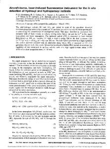
3.2 Precision VIRGAS data demonstrate that instrument precision is consistent with that expected from Poisson statistics of the PMT photon counts. Figure 11 shows an Allan deviation analysis of 1.2 hours of data from the October 28 flight in the lower stratosphere over the continental US when the SO2 mixing ratio was steady at an average of 3.1 ppt. During this segment the measured background was 240 cps / mW, the sensitivity was 2.1 cps / ppt / mW and the average laser power was 2.0 mW.

10

The precision yields a 1-σ detection limit of 2 ppt for a 10 s averaging time. The expected noise level from Poisson statistics based on these parameters shown in the figure is in excellent agreement with the observed noise level. In addition, 1-σ detection limits are shown for two published CIMS SO2 measurements (Fiedler et al., 2009; Jurkat et al., 2015) as well as the value derived in our laboratory for a Thermo Environmental Model 43C SO2 analyzer. To the best of our knowledge, the precision demonstrated in this work is the best reported precision for an ambient SO2 measurement. It is expected that

15

through achievable increases in laser power and further narrowing of the laser linewidth, the detection limit demonstrated here could improve by a factor of 2 or more. Figure 12 shows a sample of the vertical SO2 profiles acquired during VIRGAS extending from 1 km above the surface to the lower stratosphere above 19 km. This data segment is from October 28 on the final descent of the WB-57F into Ellington

20

Field. Data shown are averaged to 1 Hz at 3 km and below and averaged to 0.1 Hz above 3 km. The precision demonstrated here appears to be sufficient to resolve significant atmospheric variability and provide a comprehensive view of SO2 up to the lower stratosphere. Figure 13 shows just the segment between 12 – 17 km. The relationship observed here in the UT/LS between SO2 and O3 supports the validity of the fine-structure observed in SO2, as SO2 and O3 are anti-correlated in this region, presumably due to troposphere – stratosphere mixing in the extratropics (Pan et al., 2004).

25 4 Summary A new, in situ, LIF-based SO2 instrument has been developed and demonstrated for measurements in the UT/LS. The instrument uses a novel custom-build fiber-based laser to produce typically 2 - 4 mW of power at 216.9 nm. This power is sufficient for precise measurements at LIF cell pressures as low as 35 hPa, which is adequate for instrument operation at the 30

maximum altitudes of high-altitude research aircraft (19-20 km). The instrument is calibrated by SO2 standard addition and zeroed routinely in flight. The laboratory and flight data demonstrate that the current accuracy of the UT/LS 1 Hz measurements is ±(16 % + 0.9) ppt. Typical noise (1-σ precision) at 1 Hz was 5 - 6 ppt. Averaging the data to 0.1 Hz

13


provides a noise level of 2 ppt (1-σ precision). In-flight UT/LS measurements on and off of an SO2 resonance at 216.9 nm indicate the absence of significant interferences from other non-SO2 fluorescing species. Performance and physical specifications for the VIRGAS WB-57F instrument are summarized in Table 1. Although 5

minimizing space, weight and power requirements were important considerations in the new flight instrument, they were not optimized. A reintegration of the SO2 instrument could significantly reduce each while maintaining or improving performance. Ongoing work to improve the laser operation is expected to improve stability of the laser power and wavelength, and to provide higher signal by narrowing the laser bandwidth to match the SO2 spectrum. Interference tests with aromatics that are known to fluoresce upon excitation in this region are planned to optimize operation and constrain the

10

uncertainties when the instrument is used in polluted tropospheric regions. A series of flights with the instrument integrated on the NASA WB-57F provided valuable engineering and scientific data, with the latter providing the most comprehensive in-situ characterization of SO2 in the tropical UT/LS to date. Instrument precision appears sufficient to resolve significant atmospheric structure and hence to test global model predictions and

15

satellite retrievals of SO2 in the UT/LS. Acknowledgements This research was funded by the NOAA Atmospheric Chemistry, Carbon Cycle, and Climate Program, and the NASA Radiation Sciences Program. We would like to thank the NASA WB-57F crew and management team for support during

20

VIRGAS integration and flights. We thank K. Rosenlof, P. Newman, and E. Ray for organization and flight planning during VIRGAS.

14


References Ahmed, S. M. and Kumar, V.: Quantitative photoabsorption and flourescence spectroscopy of SO2 at 188–231 and 278.7– 320 nm, J. Quant. Spectrosc. Radiat. Transf., 47(5), 359–373, doi:10.1016/0022-4073(92)90038-6, 1992. 5

Bludský, O., Nachtigall, P., Hrušák, J. and Jensen, P.: The calculation of the vibrational states of SO2 in the C̃ 1B2 electronic state up to the SO(3Σ-)+O(3P) dissociation limit, Chem. Phys. Lett., 318(6), 607–613, doi:10.1016/S00092614(00)00015-4, 2000. Bradshaw, J. D., Rodgers, M. O. and Davis, D. D.: Single photon laser-induced fluorescence detection of NO and SO2 for atmospheric conditions of composition and pressure, Appl. Opt., 21(14), 2493, doi:10.1364/AO.21.002493, 1982.

10

Brand, J. C. D. and Srikameswaran, K.: The Π*-Π (2350 Å) band system of sulphur dioxide, Chem. Phys. Lett., 15(1), 130– 132, doi:10.1016/0009-2614(72)87034-9, 1972. Calvert, J. C., Ed.: SO2, NO and NO2 Oxidation Mechanisms: Atmospheric Considerations, 3rd ed., Butterworth Publishers, Stoneham, MA., 1984. Cazorla, M., Wolfe, G. M., Bailey, S. A., Swanson, A. K., Arkinson, H. L. and Hanisco, T. F.: A new airborne laser-induced

15

fluorescence instrument for in situ detection of formaldehyde throughout the troposphere and lower stratosphere, Atmos. Meas. Tech., 8(2), 541–552, doi:10.5194/amt-8-541-2015, 2015. Dentener, F., Kinne, S., Bond, T., Boucher, O., Cofala, J., Generoso, S., Ginoux, P., Gong, S., Hoelzemann, J. J., Ito, a., Marelli, L., Penner, J. E., Putaud, J.-P., Textor, C., Schulz, M., van der Werf, G. R. and Wilson, J.: Emissions of primary aerosol and precursor gases in the years 2000 and 1750, prescribed data-sets for AeroCom, Atmos. Chem. Phys. Discuss.,

20

6(2), 2703–2763, doi:10.5194/acpd-6-2703-2006, 2006. Digangi, J. P., Boyle, E. S., Karl, T., Harley, P., Turnipseed, A., Kim, S., Cantrell, C., Maudlin, R. L., Zheng, W., Flocke, F., Hall, S. R., Ullmann, K., Nakashima, Y., Paul, J. B., Wolfe, G. M., Desai, A. R., Kajii, Y., Guenther, A. and Keutsch, F. N.: First direct measurements of formaldehyde flux via eddy covariance: Implications for missing in-canopy formaldehyde sources, Atmos. Chem. Phys., 11(20), 10565–10578, doi:10.5194/acp-11-10565-2011, 2011.

25

Fiedler, V., Nau, R., Ludmann, S., Arnold, F., Schlager, H. and Stohl, A.: East Asian SO2 pollution plume over Europe Part 1: Airborne trace gas measurements and source identification by particle dispersion model simulations, Atmos. Chem. Phys., 9(14), 4717–4728, doi:10.5194/acp-9-4717-2009, 2009. Gao, R. S., McLaughlin, R. J., Schein, M. E., Neuman, J. A., Ciciora, S. J., Holecek, J. C. and Fahey, D. W.: Computercontrolled Teflon flow control valve, Rev. Sci. Instrum., 70(12), 4732, doi:10.1063/1.1150137, 1999.

30

Gao, R. S., Ballard, J., Watts, L. A., Thornberry, T. D., Ciciora, S. J., McLaughlin, R. J. and Fahey, D. W.: A compact, fast UV photometer for measurement of ozone from research aircraft, Atmos. Meas. Tech., 5(9), 2201–2210, doi:10.5194/amt-5-2201-2012, 2012. Heckendorn, P., Weisenstein, D., Fueglistaler, S., Luo, B. P., Rozanov, E., Schraner, M., Thomason, L. W. and Peter, T.: The Impact of Geoengineering Aerosols on Stratospheric Temperature and Ozone, Environ. Res. Lett., 4, 045108, 15


doi:10.1088/1748-9326/4/4/045108, 2011. Heidt, L. E., Vedder, J. F., Pollock, W. H., Lueb, R. a. and Henry, B. E.: Trace gases in the Antarctic atmosphere, J. Geophys. Res., 94(D9), 11599, doi:10.1029/JD094iD09p11599, 1989. Hofmann, D., Barnes, J., O’Neill, M., Trudeau, M. and Neely, R.: Increase in background stratospheric aerosol observed 5

with

lidar

at

Mauna

Loa

Observatory

and

Boulder,

Colorado,

Geophys.

Res.

Lett.,

36(15),

3–7,

doi:10.1029/2009GL039008, 2009. Hui, M.-H. and Rice, S. A.: Decay fluorescence from single vibronic levels of SO2, Chem. Phys. Lett., 20(5), 411–412, doi:10.1016/0009-2614(73)85186-3, 1973. Jurkat, T., Kaufmann, S., Voigt, C., Schäuble, D., Jeßberger, P. and Ziereis, H.: The airborne mass spectrometer AIMS - Part 10

2: Measurements of trace gases with stratospheric or tropospheric origin in the UTLS, Atmos. Meas. Tech. Discuss., 8(12), 13567–13607, doi:10.5194/amtd-8-13567-2015, 2015. Kirkby, J., Curtius, J., Almeida, J., Dunne, E., Duplissy, J., Ehrhart, S., Franchin, A., Gagné, S., Ickes, L., Kürten, A., Kupc, A., Metzger, A., Riccobono, F., Rondo, L., Schobesberger, S., Tsagkogeorgas, G., Wimmer, D., Amorim, A., Bianchi, F., Breitenlechner, M., David, A., Dommen, J., Downard, A., Ehn, M., Flagan, R. C., Haider, S., Hansel, A., Hauser, D.,

15

Jud, W., Junninen, H., Kreissl, F., Kvashin, A., Laaksonen, A., Lehtipalo, K., Lima, J., Lovejoy, E. R., Makhmutov, V., Mathot, S., Mikkilä, J., Minginette, P., Mogo, S., Nieminen, T., Onnela, A., Pereira, P., Petäjä, T., Schnitzhofer, R., Seinfeld, J. H., Sipilä, M., Stozhkov, Y., Stratmann, F., Tomé, A., Vanhanen, J., Viisanen, Y., Vrtala, A., Wagner, P. E., Walther, H., Weingartner, E., Wex, H., Winkler, P. M., Carslaw, K. S., Worsnop, D. R., Baltensperger, U. and Kulmala, M.: Role of sulphuric acid, ammonia and galactic cosmic rays in atmospheric aerosol nucleation, Nature, 476(7361),

20

429–433, doi:10.1038/nature10343, 2011. Koplow, J. P., Di Teodoro, F., Kliner, D. a. ., Moore, S. W. and Smith, A. V: Efficient second, third, fourth, and fifth harmonic generation of a Yb-doped fiber amplifier, Opt. Commun., 210(September), 393–398, doi:10.1016/S00304018(02)01825-4, 2002. Kulmala, M., Kontkanen, J., Junninen, H., Lehtipalo, K., Manninen, H. E., Nieminen, T., Petaja, T., Sipila, M.,

25

Schobesberger, S., Rantala, P., Franchin, A., Jokinen, T., Jarvinen, E., Aijala, M., Kangasluoma, J., Hakala, J., Aalto, P. P., Paasonen, P., Mikkila, J., Vanhanen, J., Aalto, J., Hakola, H., Makkonen, U., Ruuskanen, T., Mauldin, R. L., Duplissy, J., Vehkamaki, H., Back, J., Kortelainen, A., Riipinen, I., Kurten, T., Johnston, M. V, Smith, J. N., Ehn, M., Mentel, T. F., Lehtinen, K. E. J., Laaksonen, A., Kerminen, V.-M. and Worsnop, D. R.: Direct Observations of Atmospheric Aerosol Nucleation, Science, 339(6122), 943–946, doi:10.1126/science.1227385, 2013.

30

Lamarque, J.-F., Bond, T. C., Eyring, V., Granier, C., Heil, A., Klimont, Z., Lee, D., Liousse, C., Mieville, A., Owen, B., Schultz, M. G., Shindell, D., Smith, S. J., Stehfest, E., Van Aardenne, J., Cooper, O. R., Kainuma, M., Mahowald, N., McConnell, J. R., Naik, V., Riahi, K. and van Vuuren, D. P.: Historical (1850–2000) gridded anthropogenic and biomass burning emissions of reactive gases and aerosols: methodology and application, Atmos. Chem. Phys., 10(15), 7017– 7039, doi:10.5194/acp-10-7017-2010, 2010. 16


Lelieveld, J., Evans, J. S., Fnais, M., Giannadaki, D. and Pozzer, A.: The contribution of outdoor air pollution sources to premature mortality on a global scale., Nature, 525(7569), 367–71, doi:10.1038/nature15371, 2015. Manatt, S. L. and Lane, A. L.: A compilation of the absorption cross-sections of SO2 from 106 to 403 nm, J. Quant. Spectrosc. Radiat. Transf., 50(3), 267–276, doi:10.1016/0022-4073(93)90077-U, 1993. 5

Matsumi, Y., Shigemori, H. and Takahashi, K.: Laser-induced fluorescence instrument for measuring atmospheric SO2, Atmos. Environ., 39(17), 3177–3185, doi:10.1016/j.atmosenv.2005.02.023, 2005. Mauldin III, R. L., Berndt, T., Sipilä, M., Paasonen, P., Petäjä, T., Kim, S., Kurtén, T., Stratmann, F., Kerminen, V.-M. and Kulmala, M.: A new atmospherically relevant oxidant of sulphur dioxide, Nature, 488(7410), 193–196, doi:10.1038/nature11278, 2012.

10

McNutt, M. K., Abdalati, W., Caldeira, K., Doney, S. C., Falkowski, P. G., Fetter, S., Fleming, J. R., Hamberg, S. P., Morgan, M. G., Penner, J. E., Pierrehumbert, R. T., Rasch, P. J., Russell, L. M., Snow, J. T., Titley, D. W. and Wilcox, J.: Climate Intervention: Reflecting Sunlight to Cool Earth, Washington DC., 2015. Myhre, G., Shindell, D., Bréon, F.-M., Collins, W., Fuglestvedt, J., Huang, J., Koch, D., Lamarque, J.-F., Lee, D., Mendoza, B., Nakajima, T., Robock, A., Stephens, G., Takemura, T. and Zhang, H.: Anthropogenic anc Natural Radiative Forcing.

15

In: Climate Change 2013: The Physical Science Basis. Contribution of Working Group I to the Fifth Assessment Report of the Intergovernmental Panel on Climate Change, edited by T. F. Stocker, D. Qin, G.-K. Plattner, M. Tignor, S. K. Allen, J. Boschung, A. Nauels, Y. Xia, V. Bex, and P. M. Midgley, Cambridge University Press, Cambridge, UK and New York, NY, USA., 2013. Okabe, H.: Fluorescence and predissociation of sulfur dioxide, J. Am. Chem. Soc., 93(25), 7095–7096,

20

doi:10.1021/ja00754a072, 1971. Pan, L. L., Randel, W. J., Gary, B. L., Mahoney, M. J. and Hintsa, E. J.: Definitions and sharpness of the extratropical tropopause: A trace gas perspective, J. Geophys. Res. D Atmos., 109(23), 1–11, doi:10.1029/2004JD004982, 2004. Pierce, J. R., Weisenstein, D. K., Heckendorn, P., Peter, T. and Keith, D. W.: Efficient formation of stratospheric aerosol for climate engineering by emission of condensible vapor from aircraft, Geophys. Res. Lett., 37(18), 2–6,

25

doi:10.1029/2010GL043975, 2010. Randel, W. J., Park, M., Emmons, L., Kinnison, D., Bernath, P., Walker, K. A., Boone, C. and Pumphrey, H.: Asian Monsoon Transport of Pollution to the Stratosphere, Science, 328(5978), 611–613, doi:10.1126/science.1182274, 2010. Roiger, A., Aufmhoff, H., Stock, P., Arnold, F. and Schlager, H.: An aircraft-borne chemical ionization – ion trap mass spectrometer (CI-ITMS) for fast PAN and PPN measurements, Atmos. Meas. Tech., 4(2), 173–188,

30

doi:10.5194/amt-4-173-2011, 2011. Rufus, J., Stark, G., Smith, P. L., Pickering, J. C. and Thorne, A. P.: High-resolution photoabsorption cross section measurements of SO2, 2: 220 to 325 nm at 295 K, J. Geophys. Res. Planets, 108(E2), doi:10.1029/2002JE001931, 2003. Scott, S. G., Bui, T. P., Chan, K. R. and Bowen, S. W.: The Meteorological Measurement System on the NASA ER-2 Aircraft, J. Atmos. Ocean. Technol., 7(4), 525–540, doi:10.1175/1520-0426(1990)0072.0.CO;2, 1990. 17


Seinfeld, J. H. and Pandis, S. H.: Atmospheric Chemistry and Physics: From Air Pollution to Climate Change, second., John Wiley & Sons, Inc., Hoboken, New Jersey., 2006. Solomon, S., Daniel, J. S., Neely 3rd, R. R., Vernier, J. P., Dutton, E. G. and Thomason, L. W.: The persistently variable “background” 5

stratospheric

aerosol

layer

and

global

climate

change,

Science,

333(6044),

866–870,

doi:10.1126/science.1206027, 2011. Stark, G., Smith, P. L., Rufus, J., Thorne, A. P., Pickering, J. C. and Cox, G.: High-resolution photoabsorption cross-section measurements of SO 2 at 295 K between 198 and 220 nm, J. Geophys. Res. Planets, 104(E7), 16585–16590, doi:10.1029/1999JE001022, 1999. Stocker, T. F., D. Qin, G.-K., Plattner, L. V., Alexander, S. K., Allen, N. L., Bindoff, F.-M., Bréon, J. a., Church, U.,

10

Cubasch, S., Emori, P., Forster, P., Friedlingstein, N., Gillett, J. M., Gregory, D. L., Hartmann, E., Jansen, B., Kirtman, R., Knutti, K., Krishna Kumar, P., Lemke, J., Marotzke, V., Masson-Delmotte, G. a., Meehl, I. I., Mokhov, S., Piao, V., Ramaswamy, D., Randall, M., Rhein, M., Rojas, C., Sabine, D., Shindell, L. D., Talley, D. G. and Xie, V. and S.-P.: Technical Summary, Clim. Chang. 2013 Phys. Sci. Basis. Contrib. Work. Gr. I to Fifth Assess. Rep. Intergov. Panel Clim. Chang., 33–115, doi:10.1017/ CBO9781107415324.005, 2013.

15

Thornberry, T. D., Rollins, A. W., Gao, R. S., Watts, L. A., Ciciora, S. J., McLaughlin, R. J. and Fahey, D. W.: A twochannel, tunable diode laser-based hygrometer for measurement of water vapor and cirrus cloud ice water content in the upper troposphere and lower stratosphere, Atmos. Meas. Tech., 8(1), 211–224, doi:10.5194/amt-8-211-2015, 2015. Vernier, J. P., Thomason, L. W. and Kar, J.: CALIPSO detection of an Asian tropopause aerosol layer, Geophys. Res. Lett., 38(7), 1–6, doi:10.1029/2010GL046614, 2011.

20

Vet, R., Artz, R. S., Carou, S., Shaw, M., Ro, C.-U., Aas, W., Baker, A., Bowersox, V. C., Dentener, F., Galy-Lacaux, C., Hou, A., Pienaar, J. J., Gillett, R., Forti, M. C., Gromov, S., Hara, H., Khodzher, T., Mahowald, N. M., Nickovic, S., Rao, P. S. P. and Reid, N. W.: A global assessment of precipitation chemistry and deposition of sulfur, nitrogen, sea salt, base

cations,

organic

acids,

acidity

and

pH,

and

phosphorus,

Atmos.

Environ.,

93,

3–100,

doi:10.1016/j.atmosenv.2013.10.060, 2014. 25

Wennberg, P. O., Cohen, R. C., Hazen, N. L., Lapson, L. B., Allen, N. T., Hanisco, T. F., Oliver, J. F., Lanham, N. W., Demusz, J. N. and Anderson, J. G.: Aircraft-borne, laser-induced fluorescence instrument for the in situ detection of hydroxyl and hydroperoxyl radicals, Rev. Sci. Instrum., 65(6), 1858–1876, doi:10.1063/1.1144835, 1994.

18


Table 1: Performance and physical specifications for operation of the SO2 instrument the NASA WB-57F.

Size

86 x 60 x 34 cm

Weight

90 kg

Max. Power

Instrument: 300 W Pump: 300 W Heaters: 800 W

1-σ Precision

2 ppt, 10 s

Accuracy

±(16 % + 0.9 ppt)

Time Response

0.1 s

19


5

10

Figure 1: SO2 absorption spectrum compiled by Manatt and Lane (1993). The approximate region used in lamp based SO2 fluorescence instrumentation (205 – 220 nm) is indicated by the shaded gray region, and the 216.9 used in this work indicated by the solid violet line. Spectral regions used by OMI (Ozone Monitoring Instrument) and SCIAMACHY (Scanning Imaging Absorption Spectrometer for Atmospheric Cartography) satellite instruments for column SO2 retrievals are indicated. Bands corresponding to excitations into the first three electronic excitations of SO2 are indicated by ã, B̃ , and C̃ .

Figure 2: Schematic of the relevant SO2 electronic structure and LIF process. Excitation from the ground state, X̃ , to above the dissociation threshold in the C̃ state at 216.9 nm (purple line) leads to predissociation in the majority of SO2 molecules. A small fraction undergo internal vibrational relaxation (dashed blue arrow) followed by red-shifted fluorescence (red arrows).

20


Figure 3: Schematic of the fiber-amplified diode laser system at 1084.5 nm. See text in Section 2.2 for detailed explanation.

5 Figure 4: Optics bench photo. Dashed pink line indicates 217 nm beam path. Labeled parts: 1) fiber output, 2) nonlinear crystals, 3) Pellin-Broca prism, 4) PMT, 5) sample inlet, 6) main exhaust, 7) SO2 reference cell, 8) Photodiodes, 9) PAD.

21


5

10

Figure 5: Count rate linearity adjustment. (Top) Calculated relationship between observed and true photon count rates from Eq. (1) assuming a 25 kHz laser pulse frequency and a maximum of 1 count / laser pulse. (Bottom) Fraction of increased signal observed as a function of the true count rate (O). Bottom axis (SO2) is calculated from the top axis assuming 300 cps background and 7 cps / ppt signal.

Figure 6: Schematic of flow and calibration system. Red line indicates the main inlet, which was housed in a pylon extending 28 cm below the WB-57F skin, and heated to 45 °C. Blue lines indicate components at vacuum (< 5 hPa). Excluding the components in the inlet pylon, all instrument components were housed in an insulated enclosure maintained at 20 - 30 °C.

22


Figure 7: Example in-flight SO2 calibration during the flight of October 28, 2015. Data shown are the linearized count rate divided by the measured laser power. The dashed line shows a fit to the 4 data points indicating the sensitivity of 3.5 cps / mW / ppt and background of 150 cps / mW.

5

Figure 8: Example of the instrument time response following the removal of calibration gas from the instrument sample line. The dashed line is an exponential decay with a time constant of 0.1 s.

23


5

10

Figure 9: Example of observed signal during a scan of the laser when sampling 3.4 ppb SO2 from a gas standard during a WB-57F flight. The black line plotted on the left axis shows the literature SO2 absorption cross section. Plotted in red against the right axis is the observed signal from the LIF system. Red dash line shows typical signal observed when scanning laser with a zero-air sample.

Figure 10: Data sample from flight on Oct. 27, 2015. Top panel shows ambient pressure, indicating a cruise in the lower stratosphere followed by descent into the upper troposphere. Bottom panel: Gray shows 5 Hz data. Black, red, cyan and green show 1 Hz averages of ambient sampling, calibration, laser wavelength scan, and zero-air zeroing.

24


5

Figure 11: Instrument precision (Allan deviation) during a 1.2 hour segment sampling an average SO2 abundance of 3.1 ppt in the LS during the Oct. 28 flight compared to the expected precision (Poisson limit). Other points show 1-σ precision values for a commercial pulsed-fluorescence instrument (TECO) and two CIMS instruments (Jurkat et al., 2015; Roiger et al., 2011).

10

Figure 12: Data from final descent on Oct. 28. Left panel: 10 s averages shown above 3 km, 1 s averages shown below 3 km. Gaps in the SO2 data are during periods where instrument calibrations and zero measurements occurred.

25


Figure 13: Data from final descent on Oct. 28 in the range 12 – 17 km.

26