Aug 14, 2017 - realistic neuronal dynamics [12] and stochastic synapses [13, 14]. Establishing a link between ... 1. arXiv:1708.04251v1 [cs.NE] 14 Aug 2017 ...
A learning framework for winner-take-all networks with stochastic synapses
arXiv:1708.04251v1 [cs.NE] 14 Aug 2017
Hesham Mostafa and Gert Cauwenberghs Institute of Neural Computation University of California San Diego {hmmostafa,gert}@ucsd.edu Abstract Many recent generative models make use of neural networks to transform the probability distribution of a simple low-dimensional noise process into the complex distribution of the data. This raises the question of whether biological networks operate along similar principles to implement a probabilistic model of the environment through transformations of intrinsic noise processes. The intrinsic neural and synaptic noise processes in biological networks, however, are quite different from the noise processes used in current abstract generative networks. This, together with the discrete nature of spikes and local circuit interactions among the neurons, raises several difficulties when using recent generative modeling frameworks to train biologically motivated models. In this paper, we show that a biologically motivated model based on multi-layer winner-take-all (WTA) circuits and stochastic synapses admits an approximate analytical description. This allows us to use the proposed networks in a variational learning setting where stochastic backpropagation is used to optimize a lower bound on the data log likelihood, thereby learning a generative model of the data. We illustrate the generality of the proposed networks and learning technique by using them in a structured output prediction task, and in a semi-supervised learning task. Our results extend the domain of application of modern stochastic network architectures to networks where synaptic transmission failure is the principal noise mechanism.
1
Introduction
The hypothesis that sensory perception is a process of active inference is key to explaining various perceptual phenomena [1, 2]. One form of this hypothesis is that the brain maintains a probabilistic model of the environment which it then uses to infer latent causes and to fill missing or ambiguous details in the noisy sensory input it receives [3]. Traditionally, there has been a clear distinction between probabilistic modeling approaches developed based on practical considerations [4, 5, 6, 7], and probabilistic models developed as mechanistic explanations of how the brain represents and manipulates probability distributions [8, 9, 10]. While the later models are more biologically relevant, they lack the scalability and power of the former. Finding a middle ground between these two types of models could prove useful in two ways: insights gained from developing practical, large-scale, and biologically-motivated generative models could shed some light on how the brain is able to model complex high-dimensional distributions, and the constraints imposed by the biological substrate could inform the development of more computationally efficient types of generative models. One example of an attempt to find such a middle ground used stochastic spiking networks to implement and sample from Boltzmann machines [11]. This model was developed further through the use of more realistic neuronal dynamics [12] and stochastic synapses [13, 14]. Establishing a link between Boltzmann machines and the dynamics of biologically realistic networks, however, is difficult due to the need for a symmetric synaptic connectivity matrix. Moreover, generating samples from the Boltzmann distribution embodied by the spiking network (either unconditional samples or samples from the posterior distribution) requires running the network for several steps in order to approach the equilibrium distribution. For highly multi-modal distributions, significant number of steps might be needed for the Markov chain to mix, making it computationally expensive to sample from the network. Restricted Boltzmann machines were among the first large-scale, effectively trainable generative models [4, 15]. Recently, however, effective variational training methods have been developed for training generative architectures with a feed-forward hierarchical structure of latent variables [6, 16] where generative samples can be obtained in a single pass through the network. Recent variational methods rely on having an analytically tractable distribution over the variables in one layer conditioned on their parent variables in the previous layer. For continuous latent variables, the distributions are typically Gaussians whose mean and variance are functions of the parent variables, while categorical/discrete variables typically follow a softmax distribution. Such distributions do not map naturally onto the dynamics of biologically-realistic networks. Moreover, they are not computationally cheap as they involve multiplications and exponentiation operations. 1
The main contribution of this paper is the development of an analytically tractable approximation of the probability distribution over possible network states in multi-layer networks of winner-take-all (WTA) circuits, where neurons in different WTA circuits are connected using stochastic synapses. Since the state of each WTA is a discrete variable, and we use samples from these discrete variables/WTAs to approximate various intractable expectations, we need to be able to backpropagate error information through these stochastic samples. The approximate expression for the probability distribution over network states that we develop allows us to make use of the recently-introduced Gumbel-softmax approximate reparameterization of discrete distributions [17, 18] to enable backpropagation through stochastic network samples. We thus obtain a general learning framework for WTA networks with stochastic synapses that can be applied to a wide range of learning problems. We first use the proposed networks in a feedforward configuration to solve a structured output prediction task in order to illustrate the soundness of our network approximation and of the training method. We then apply the proposed learning framework to learning a generative model of the MNIST dataset using variational methods. Following recent trends in variational methods, we use a stochastic neural network to implement the variational posterior. The network we use to approximate the posterior distribution over the latent variables is also based on WTA circuits with stochastic synapses. Both the generative/decoder branch and the inference/encoder branch of the network are thus composed solely of discrete valued WTA circuits. To illustrate the generality of the proposed networks, we also use them in a configuration that is inspired by ladder networks [19] to solve a semi-supervised learning task.
2
Model description
We investigate multi-layer networks of WTA circuits which have the general structure shown in Fig. 1. The network in Fig. 1 has L layers where each layer can have a different number of WTA circuits. WTA circuits in the same layer all have the same number of neurons. This number may be different in different layers. Exactly one neuron in a WTA circuit spikes during one pass through the network and this is the neuron receiving the largest input among the WTA neurons. Neurons are connected using stochastic synapses where each synapse has an independent probability to fail to transmit a spike. Let tl be the vector representing the total input to the neurons in layer l and zl a binary 0/1 vector indicating whether each neuron in layer l has spiked (1) or not (0). Let U l (i) be a function that maps a neuron index i in layer l to the set of indices of all the neurons in the same WTA. tl and zl are then given by tl = (Wl+1 ◦ Bl+1 )zl+1 1 if tli = max tlj j∈U l (i) zil = 0 otherwise
l = 0, . . . , L − 1
(1a)
l = 0, . . . , L − 1,
(1b)
where zil , tli are the ith elements in vectors zl and tl respectively. Wl is the weight matrix from layer l to layer l − 1 and Bl is a matrix of independent 0/1 Bernoulli random variables which is multiplied l element-wise with Wl . Each element � in � B can have a different probability of being 1. These probabilities are given by the matrices Zl = E Bl . Each connection thus has an independent probability to fail to transmit a spike. The lowest layer is the data layer, z 0 ≡ x. Note that network evaluation proceeds layer by layer and is thus an abstraction of the behavior of a dynamical spiking network. We assume each neuron in the top layer has an equal probability to win the competition in its WTA circuit. This prior on the top layer activity, together with the network weights and synaptic transmission failure probabilities implicitly define a probability distribution over the spike configurations generated by the network. This distribution can be written as X � � � L−1 � log Pθ (zL , zL−1 , . . . , z1 , x) = log P (zL ) + log Pθ (x | z1 ) + log Pθ (zl | zl+1 ) ,
(2)
l=1
where θ is the collection of all the network parameters (weights and transmission failure probabilities), and P (zL ) is the prior distribution over the top layer activity. It is easy to generate samples from the distribution given in Eq. 2 by sampling the top-layer prior and the failure probabilities of all the connections, then executing one pass through the network. In order to
2
all-to-all synaptic connections with stochastic transmission failures
....
...
....
.... ...
....
...
....
....
winner-take-all circuit of spiking neurons
....
....
....
Figure 1. A multi-layer network of WTA circuits. Neurons project to neurons in the next layer through stochastic connections. Exactly one neuron generates a spike in each WTA during one pass through the network. efficiently train these networks to optimize various expectations over the spike patterns generated by the network, we need to be able to quickly evaluate the probability of particular spike patterns, i.e, we need an explicit expression for the distribution in � Eq. 2. This means we need an explicit expression for the log conditional distributions log Pθ (zl | zl+1 ) . We derive this expression in the next subsection.
2.1
Deriving the conditional distribution of the latent variables
We consider a single WTA with C neurons. The WTA has C possible outputs where each output corresponds to a different neuron winning the competition and generating a spike. A neuron wins the competition in a WTA if it receives the largest input among the WTA neurons. Let ti be the input to the ith neuron of the WTA and zin the binary vector representing the input spike activity from the preceding layer. ti and its first two moments are given by ti = (wi ◦ bi )T zin
(3) T in
µ(ti ) = E [ti ] = (wi ◦ ζi ) z � � σ 2 (ti ) = E (ti − µ(ti ))2 = (wi 2 ◦ ζi ◦ (1 − ζi ))T zin ,
(4) (5)
where wi is the input weight vector for neuron i in the WTA. bi is a vector of Bernoulli random variables which model stochastic transmission failures and whose mean is ζi = E [bi ]. bi is multiplied element-wise by wi . The mean and variance of ti are given by Eqs. 4 and 5 respectively. We make use of the central limit theorem to approximate the probability distribution of ti (which is the sum of many independent random variables) by a Gaussian having the same mean and variance. This approximation is quite accurate when the total number of non-zero inputs to the neuron is large. This is the number of non-zero entries in zin which corresponds to the number of WTAs in the preceding layer. Figure 2 illustrates how the number of non-zero inputs affects the quality of the Gaussian approximation. For 10 and 20 inputs, the discrete nature of the neuron’s input distribution is evident as there are only 210 and 220 possible inputs, respectively, corresponding to the possible configurations of synaptic transmission failure. For 50 inputs, the input distribution becomes much smoother and the Gaussian approximation becomes more accurate. We first consider a WTA with two neurons whose total inputs are t1 and t2 . The probability that t1 > t2 is the probability that t1 takes a particular value multiplied by the probability that t2 takes a smaller value, averaged across all values. Alternatively, the probability that t1 > t2 is the probability that r = t1 − t2 > 0. Following the Gaussian approximation of t1 and t2 , r is also a Gaussian with mean
3
µ(t1 ) − µ(t2 ) and variance σ 2 (t1 ) + σ 2 (t2 ). The two equivalent ways of formulating P (t1 > t2 ) are thus Z ∞ φ (x; µ(t1 ), σ(t1 )) cdf (x; µ(t2 ), σ(t2 )) dx (6) P (t1 > t2 ) = −∞ ! µ(t1 ) − µ(t2 ) P (t1 > t2 ) = P (r > 0) = cdf p ; 0, 1 (7) σ 2 (t1 ) + σ 2 (t2 ) (x−µ)2 1 φ (x; µ, σ) = √ e− 2σ2 σ 2π Z x (y−µ)2 1 e− 2σ2 dy. cdf (x; µ, σ) = √ σ 2π −∞ For a WTA with C neurons whose total inputs are t1 , . . . tC , and following the same reasoning as Eq. 6, the probability that neuron i receives the largest input is Z ∞ ^ Y pi = P ( ti > tj ) = φ (x; µ(ti ), σ(ti )) cdf (x; µ(tj ), σ(tj )) dx. (8) −∞
j6=i
j6=i
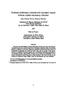
The integration in Eq. 8 is analytically intractable for C > 2. For C = 2, pi reduces to the expressions in Eqs. 6 and 7 . To approximate the integration in Eq. 8, we approximate the product of the cdf functions by one of the cdf functions making up the product. That will usually be the cdf of the Gaussian having the largest mean. This approximation is illustrated in Fig. 3. The quality of the approximation improves when the means of the Gaussians are well separated and the Gaussians have low variance. This approximation is equivalent to approximating Eq. 8 as the minimum probability that neuron i wins a pairwise competition (governed by Eqs. 6 and 7) with another neuron in the WTA: �Z ∞ � pˆi = min φ (x, µ(ti ), σ(ti )) cdf (x; µ(tj ), σ(tj )) dx (9) j6=i −∞ ( !) µ(ti ) − µ(tj ) = min cdf p ; 0, 1 (10) j6=i σ 2 (tj ) + σ 2 (ti ) pˆi p˜i = P . pˆi
(11)
j
In other words, we approximate the probability that a neuron in a WTA wins the competition (receives the largest input) by the probability that it wins the competition against one other neuron, where this other neuron is selected to be the neuron which has the highest probability to receive a larger input than the first neuron. This approximation works in practice because winning the competition against the neuron that has the highest mean input implies winning the competition against other neurons as well with a high probability. This approximation yields an unnormalized probability pˆi . The normalized probability that neuron i wins the competition is given by p˜i . Equations 4, 5, 10, and 11 define an analytical, differentiable approximation to the probability of a neuron winning the competition in a WTA given the input layer binary activity vector zin . Since the WTAs in a layer are conditionally independent given the input layer activity, these equations allow us to obtain a differentiable expression for the winning probability of all the neurons in a layer with multiple WTAs. In a layer with multiple WTAs, and where p˜i is the probability that neuron i wins the competition in its WTA given the input layer activity zin , the log probability of observing a particular spike pattern zout (which is a 0/1 binary vector) is � X log p(zout | zin ) = log(p˜i )ziout . (12) i
zout has to be a valid spike pattern, i.e, with exactly one neuron in each WTA emitting a spike. Our approximation of a layer’s conditional distribution can be used to obtain an explicit expression for the distribution in Eq. 2.
4
1.8 1.6 1.4 1.2 1.0 0.8 0.6 0.4 0.2 0.0 10 0.30
Probability
Probability
Probability
Gaussian approximation Total input histogram
10 inputs 5
0
5
10
15
Gaussian approximation Total input histogram
0.25 0.20 0.15
20 inputs
0.10 0.05 0.00 10 0.12
5
0
5
10
15
Gaussian approximation Total input histogram
0.10 0.08 0.06
50 inputs
0.04 0.02 0.00 15
10
5
0
5
Total neuron input
10
15
20
Figure 2. Quality of the Gaussian approximation of the neuron’s input distribution. We considered a neuron with 10, 20, and 50 inputs. The inputs are all 1s. The input connection weights were drawn randomly from a standard normal distribution. Each connection has an independent probability to fail which is drawn uniformly at random from [0, 1]. After fixing the connection weights and failure probabilities, we generate 500000 samples for each of the three input sizes to construct the total input histogram.
2.2
Reparameterizing the latent variables distribution
When training stochastic WTA networks containing latent variables z, we typically need to evaluate expectations of the form EPθ (z|x0 ) (f (z, x0 )), where Pθ (z | x0 ) is the probability distribution over the latent variables given an observed data point x0 ; θ is the vector of network parameters (synaptic weights and transmission failure probabilities) which implicitly define the distribution P ; and f is a differentiable function of z and x0 . f can be for example the log probability of observing a particular configuration of latent variables, or it can be a variational lower bound on the data log-likelihood. Exact evaluation of this expectation is typically intractable so it is often approximated using N samples from Pθ (z | x0 ): EPθ (z|x0 ) (f (z, x0 )) ≈
1 N
X
f (zi , x0 ).
(13)
zi ∼Pθ (z|x0 )
In order to use gradient descent to maximize or minimize this expectation with respect to the the parameters θ, we need to be able to estimate ∇θ EPθ (z|x0 ) (f (z, x0 )). Evaluating these derivatives is also analytically intractable so we have to resort to sampling approaches. One of the classical algorithms for estimating gradients of stochastic expectations with respect to the parameters of the expectation probability density is the REINFORCE algorithm [20]. Recently, however, better estimators with greatly reduced variance have been introduced [6, 16, 21]. These estimators make use of the so-called ‘reparameterization trick’ which is illustrated in Fig. 4. Through reparameterization, samples from a probability distribution can be written as a differentiable transformation of the distribution parameters and stochastic samples from a fixed standard distribution. Thus, one can directly use the chain rule to obtain the derivative of the sample-based estimate of the expectation in Eq. 13 with respect to the distribution parameters θ since f is differentiable, and through the reparameterization trick, we have a differentiable relation between the stochastic samples zi and the distribution parameters θ. Not all distributions admit such a reparameterization. Most notably, reparameterizations of discrete distributions can not be differentiable. An approximate differentiable reparameterization that works well in practice is the Gumbel-softmax reparameterization [17, 18] which we reproduce below. Given a discrete distribution described by the probability vector p = [p1 , . . . , pK ] defining the probability of each of the 5
cumulative probability
1.0 cdf1 cdf2 cdf3 cdf4 product of cdfs
0.8 0.6 0.4 0.2 0.0 10
5
0
5
10
15
cumulative probability
1.0 0.8
cdf1 cdf2 cdf3 cdf4 product of cdfs
0.6 0.4 0.2 0.0 10
5
0
5
random variable
10
15
Figure 3. Approximating the product of four cumulative density functions (dashed black line) by one of the cumulative density functions making up the product. In the top plot, this product is approximated reasonably well by cdf 4. In the bottom plot, the approximation by cdf 4 is worse due to the larger variance of some of the cumulative density functions. distribution’s K outcomes, a sample can be drawn from this discrete distribution using the following non-differentiable reparameterization: ˜ z = one_hot(arg max(gj + log(pj ))).
(14)
j
˜ z is a one-hot vector with exactly one-entry equal to one and the others zero. The index of this entry is the sample outcome and is given by the arg max operator. g1 , . . . , gK are independent samples from the Gumbel(0, 1) distribution [22]. Samples from Gumbel(0, 1) can be obtained by first sampling from the uniform distribution uj ∼ U nif orm(0, 1) and then transforming the uniform samples using gj = −log(−log(uj )). ˜ z is a one-hot K − dim vector that can take one of K possible values. In order to obtain a continuous differentiable reparameterization, the arg max operator is relaxed to the differentiable sof tmax function: exp((gj + log(pj ))/τ ) j = 1, . . . , K. (15) zˆj = PK l=1 exp((gl + log(pl ))/τ ) The sample vector ˆ z = [ˆ z1 , . . . , zˆK ] is now differentiable with respect to the parameters of the discrete distribution, p. ˆ z is a sample from a continuous distribution that approaches the original discrete distribution as the temperature parameter τ approaches 0. While training the network, τ is gradually annealed towards 0. Instead of sampling zi directly from Pθ (z | x0 ), we use the probabilities of the different discrete states of each WTA (given by Eqs. 4, 5, 10, and 11) in Eq. 15 to sample the WTA states, and use the resulting reparameterized continuous-valued samples, ˆ zi , to evaluate the expectation in Eq. 13. When sampling from multi-layer networks such as the network in Fig. 1, we use the reparameterized continuous-valued samples of one layer to evaluate the winning probabilities of the WTAs in the next layer, and then use these winning probabilities to obtain reparameterized continuous-valued samples from the next layer. We do this layer by layer until we obtain reparameterized continuous-valued samples of all the WTAs in the network. In the exact case, only one neuron can win the competition in a WTA. Samples obtained using the continuous relaxation in Eq. 15, however, yield a continuous-valued activity vector for the WTA circuit, where neurons that have a higher probability of winning are more likely to have higher activities in the sample vectors. This can be understood as approximating the hard WTA circuit by a soft WTA circuit [23] where the winning neuron does not completely shut down the activity in the other WTA neurons. We 6
sample
reparameterize
sample
fixed distribution Figure 4. The reparameterization of probability distributions to obtain a differentiable relation between the samples and the distribution parameters. Instead of sampling directly from a distribution (left), the distribution is reparameterzied so that a sample can be obtained using a differentiable deterministic transformation, g, where randomness is injected using stochastic samples �˜ from a fixed distribution (right). This results in a differentiable pathway from the stochastic sample z˜ to the distribution parameters θ and the conditioned variable x. For example, instead of sampling directly from a Gaussian z˜ ∼ N (z; µ(θ, x), σ(θ, x)), we sample first from a standard normal distribution �˜ ∼ N (�, 0, 1) then obtain z˜ using z˜ = g(x, θ, �˜) = µ(θ, x) + �˜σ(θ, x)) only use this soft WTA mechanism during training to allow gradients to flow back through stochastic samples. During testing, we use the hard WTA mechanism where only the neuron receiving the largest input emits a spike, and use the exact network dynamics with stochastic synaptic transmission failures to generate samples from the network instead of the approximation in Eq. 11. All experiments were carried out using Theano [24, 25], and all loss functions were optimized using ADAM [26].
3 3.1
Results Structured output prediction
We first validate the soundness of our approximation of the WTA winning probabilities in a structured output prediction task where the goal is to predict the lower half of an MNIST image given the upper half. The MNIST dataset contains 70000 28 × 28 grayscale images of handwritten digits split into three groups of 50000, 10000, and 10000 images for training, validation, and testing respectively. As in ref. [27, 28], we use a binarized version of the MNIST images obtained by thresholding the pixel intensities. We use a feedforward network illustrated in Fig. 5a to predict the lower image half. We represent the binary inputs and outputs using WTA circuits with 2 neurons where the spike from one neuron codes for binary 0 and the spike from the other neuron for binary 1. Given a training pair xlower and xupper , the goal is to maximize the log probability of predicting the lower image half given the upper half, log(Pθ (y = xlower | x = xupper )), across all training pairs where Pθ is the probability distribution encoded by the network in Fig. 5a . Exact evaluation of this training quantity would require marginalizing over the hidden variables z1 and z2 . Instead, we estimate it using N samples from the hidden variables per example: 1 N
X
log(Pθ (y = xlower | z2i )),
(16)
z1i ∼Pθ (z1 |xlower ),z2i ∼Pθ (z2 |z1i )
where we use N = 1 sample during training. We generate samples using the continuous reparameterization from Eq. 15. This way we can backpropagate errors through these samples to the network parameters and to samples from earlier layers. During testing, we generate 100 samples using the hard WTA mechanism and the exact network dynamics with synaptic transmission failure instead of the approximate analytical distribution used during training. These samples are then used to evaluate the log likelihood of the lower half of the image given the upper half. During training, we use an annealing schedule to lower the temperature of the softmax used to approximate the hard WTA mechanism. The learning rate also decays during training. The validation set was used to tune the temperature and learning rate schedules. Even though synaptic transmission failure can be a trainable parameter, we kept it fixed at 0.5 for all synapses and only train the synaptic weights. The network achieves a test set negative log likelihood of 61.8 ± 0.074 nats (mean and standard 7
392x2 200x10 200x10 392x2 (a)
(b)
Figure 5. (a) Network used in structured output prediction task. An A×B layer is a layer with A WTAs and B neurons in each WTA. (b) Network prediction of the lower half of sample test digits. Each digit prediction used 100 samples generated using the exact network dynamics, i.e, using 100 random failure configurations for the network synapses. The horizontal lines separate the input image half (upper half) from the predicted half (lower half). deviation from 10 runs, evaluated using 100 samples for each example). This is slightly worse than the test set negative log likelihood of 58.5 nats achieved with previous stochastic networks [17] that use discrete neural variables with activation noise rather than synaptic transmission noise. We investigated whether this is due to the discrepancy between the approximate probability distribution used during training (Equations 4, 5, 10, and 11) and the intractable exact distribution induced by synaptic transmission failure which is sampled during testing; we evaluated the test set negative log likelihood using the approximate distribution used during training and it is 60.1 ± 0.067. The network thus performs better on the test set using the approximate distribution used during training. The difference in performance is slight, however, indicating that the approximation distribution reasonably matches the exact distribution over the test set, and that effective learning can be achieved using the approximate distribution. Figure 5b shows some examples of the network prediction of the lower halves of MNIST test set digits.
3.2
Learning generative models using variational autoencoders
Our goal is to learn a generative model for a set of data points with discrete values X = {x1 , x2 , . . . , xN } where xi ∈ {1, 2, . . . , k}D . We use a feedforward network of WTA circuits connected by stochastic synapses to encode the generative distribution. This is the generation network shown in Fig. 6a. We lump all the latent variables together in one vector z = [z1 , . . . , zL ] and the distribution over the network spike patterns is given by Pθ (x, z) where θ represents the generation network parameters. For the prior on the top layer variables, zL , we choose the uniform prior where each neuron has the same probability to win the competition in its WTA. Our goal is to maximize the data log likelihood log(Pθ (X)). We use variational methods to maximize this likelihood. For a particular input point, x, � � X X Pθ (x, z) log(Pθ (x)) = Pθ (z | x) log(Pθ (x)) = Pθ (z | x) log . (17) Pθ (z | x) z z Pθ (x, z) is easy to evaluate using Eqs 2 and 12. The posterior distribution Pθ (z | x) is, however, intractable. We approximate the intractable posterior by the parameterized distribution Qφ (z | x). We use a multi-layer network of WTAs connected using stochastic synapses to implement Qφ (z | x). This is the inference/recognition network shown in Fig. 6a. It has an analogous structure to the generation network except that the connections between layers are going in the opposite direction. The weights and synaptic transmission failure probabilities in the two networks are independent. Given x, the inference network induces a probability distribution Qφ (z | x) over the latent variables which can be expressed in an analogous fashion to the generative distribution using Eqs. 2 and 12. The distribution parameters φ are the weights and synaptic transmission failure probabilities in the inference network. Note that unlike
8
all-to-all synaptic connections with stochastic transmission failures Generation network:
....
winner-take-all circuit of spiking neurons
Inference network:
...
....
....
...
....
.... ...
....
.... ...
....
...
....
....
....
....
....
....
(a)
(b)
Figure 6. (a) Structure of the variational auto-encoder network. The generation network is used to generate samples from the data distribution, while the inference network is used to generate samples from the approximate posterior distribution of the latent variables given x. Both the generation and inference networks are composed solely of WTA circuits connected using stochastic synapses. No real-valued neurons or deterministic layers are used. (b) Digits generated using the generative network of a variational auto-encoder with separate style and label WTAs in the top layer while varying the values of the label and style WTAs. Each digit is constructed by fixing the top layer activity, then averaging across 300 samples. typical variational auto-encoder architectures, the latent variable layers are directly connected and there are no deterministic layers in the network. The data log-likelihood can be written as � Pθ (x, z) Qφ (z | x) log(Pθ (x)) = Qφ (z | x) log Pθ (z | x) Qφ (z | x) z � � X Pθ (x, z) = KL(Qφ (z | x)kPθ (z | x)) + Qφ (z | x) log Qφ (z | x) z X
�
= KL(Qφ (z | x)kPθ (z | x)) + L(x; θ, φ).
(18) (19) (20)
KL is the Kullback-Leibler divergence between two distributions and�i since it is non-negative, L is a lower h � Pθ (x,z) bound on the data log-likelihood given by L = EQφ (z|x) log Qφ (z|x) . Since it is intractable to evaluate L exactly due to the required summation over all z, we approximate it using N samples from the inference
9
network: 1 L≈ N
�
X
log
zi ∼Qφ (z|x)
Pθ (x, zi ) Qφ (zi | x)
� .
(21)
We maximize this sample-based lower bound through gradient descent on the parameters θ and φ, where we use the differentiable Gumbel-softmax reparameterization described in section 2.2 to backpropagate errors through the stochastic samples. A common problem with training variational auto-encoders with multiple layers of stochastic hidden variables is the collapse of the latent approximate posterior Qφ (z | x) towards the latent prior Pθ (z) which stops the latent variables in upper layers from encoding information about the input during training [29, 30]. We adopt the solution proposed in ref. [29] in which we initially only maximize the reconstruction likelihood and gradually morph the cost function to optimize the variational lower bound L. Our optimization objective is thus � � X � 1 Pθ (zi ) , (22) J = log Pθ (x | zi ) + β log N i Qφ (zi | x) z ∼Qφ (z|x)
where β gradually increases from 0 to 1 during training. When β = 1, J is equivalent to the right-hand side of Eq. 21, i.e, it becomes a sample-based estimate of L. We apply the variational auto-encoder network based on WTA circuits and stochastic synapses to learning a generative model of MNIST digits. As in the structured output prediction task, we anneal the temperature of the softmax used in the Gumbel-softmax continuous reparameterization as well as the learning rate during training. We use N = 1 samples per data point during training. We trained a network with three stochastic hidden layers of sizes 10×10, 20×10, and 30×10 going from the deepest layer downward (An A×B layer has A WTAs with B neurons in each WTA) in order to learn a generative model of the training set of MNIST digits. These layers were followed by the visible layer of 784×2 neurons. We used a uniform prior in the top layer where each neuron has an equal chance to win the competition in its WTA and used a fixed transmission failure probability of 0.5. After training, we evaluated the variational lower bound using the approximate distribution over WTA winners and N = 50 samples in Eq. 21. The samples were also drawn from the approximate distribution. This evaluation was done on the test set. Under the approximate distribution, we obtain a variational lower bound of −98.9 ± 0.3 nats (mean and standard deviation from 10 runs) which is on par with discrete stochastic neural networks that use activation noise rather than synaptic transmission noise [17]. Estimating the variational lower bound using the exact network dynamics is particularly difficult in our case as exact evaluation of Pθ (x, z) and Qφ (z | x) is intractable. Theoretically, we can estimate these probability distributions using samples, but we observed that the number of samples needed to reliably estimate the exact Pθ (x, z) and Qφ (z | x) is computationally prohibitive. Note that this problem does not arise in conventional variational auto-encoders as they have exact expressions for the conditional log probability of each layer’s activity. There are two steps to our approximation of the winning probability of the neurons in a WTA: the first step assumes the input to each neuron is Gaussian, the second step approximates the intractable integration in Eq. 8 with the tractable integration in Eq. 9. The first step is practically unavoidable, as the exact distribution of the input to a neuron is an intractable discrete distribution where each point corresponds to one configuration of synaptic failures. We can dispense with the second step, however, by numerically evaluating the integration in Eq. 8. Our estimate of the variational lower bound that is more faithful to the exact network dynamics uses exactly generated samples zi in Eq. 21, i.e, samples of z generated by sampling the synaptic transmission failure probabilities, and it uses numerical integration of Eq. 8 to obtain accurate winning probabilities in each WTA. The accurate winning probabilities are used to evaluate Pθ (x, z) and Qφ (z | x). Under this estimate, the variational lower bound is −104 ± 1.4 nats which is slightly worse than the lower bound evaluated using the approximate distribution used during training. We trained another variational auto-encoder network in which a subset of the WTAs in the top layer were forced to represent the MNIST image label. The network had three stochastic hidden layers of sizes 20×10, 30×10, and 30×10 going from the deepest layer downward. The top layer prior used during training was label dependent: 5 of the 20 WTAs in the top layer had a delta function prior centered on the neuron whose index corresponds to the label of the current training example, while the remaining 15 WTAs used a uniform prior. During training, different values of the top 15 WTAs with uniform prior will represent different variants of each digit (where the digit is specified by the other 5 WTAs). Aesthetically, 10
each configuration of the 15 WTAs will give rise to 10 digits (0 to 9) having similar style. We chose 5 WTAs to represent the label in order to have a significant label-dependent part in the top layer activity. After training, we sample from the generative network by forcing the 5 label WTAs to represent one label and randomly choosing a winner in the remaining 15 WTAs in the top layer, i.e, we choose a label and a random style. We then sample from the remaining layers using the exact network dynamics. The sampled images are shown in Fig. 6b.
3.3
Semi-supervised learning using ladder networks
Noise plays a crucial role in several auto-encoding architectures [31, 32, 33] where it limits the information flowing between network layers, thereby forcing networks to learn more compact and general representations in an unsupervised manner. In a semi-supervised setting, the representations learned in an unsupervised manner are fed to a classifier and few labeled examples are used to train the classifier (and the underlying representations as well). By simultaneously learning representations to optimize the unsupervised loss (reconstruction error) and the supervised loss (label prediction error), the network can learn to extract the label-relevant information using only few labeled examples. We used WTA networks with stochastic synapses to construct an auto-encoder and added a linear classifier on top of the deepest hidden layer. We applied this architecture to an MNIST semi-supervised learning task where only a subset of the labeled examples from the training set were used to train the classifier. The full (unlabeled) training set was used to train the auto-encoder. We used a ladder architecture [19] for the auto-encoder as shown in Fig. 7 with lateral connections between the encoding and decoding branches. In the original ladder networks [19], the real-valued activations in the encoding branch (leftmost branch in Fig. 7) are corrupted through the addition of Gaussian noise. In our case, the corruption of the encoding branch is achieved through the use of stochastic synapses. The parallel, uncorrupted branch providing the reconstruction targets (rightmost branch in Fig. 7) uses deterministic synapses and the same weight matrices as the corrupted encoding branch. For each training example, the encoding branch and reconstruction branch are sampled to obtain p ˆx , p ˆ 1 , and p ˆ 2 which are the probability vectors for generating a spike in the reconstruction branch layers. x, z1 , and z2 are the binary spike vectors in the corresponding layers in the clean input branch. The unsupervised reconstruction loss is then given by Lunsupervised = − (< x, log(ˆ px ) > + < z1 , log(ˆ p1 ) > + < z2 , log(ˆ p2 ) >) ,
(23)
where is the dot product operator. y is the input vector to the top classifier layer. The supervised loss at the classifier layer is the cross-entropy loss: exp(yr ) , Lsupervised = −log P exp(yi )
(24)
i
where r is the input label index. During training, a fixed labeled subset of the training set is used to minimize Lsupervised while the full training set was used to minimize Lunsupervised . As in previous experiments, we anneal the temperature of the softmax used in the Gumbel-softmax continuous reparameterization as well as the learning rate during training, and keep synaptic failure probabilities fixed at 0.5. When classifying the test set, a deterministic version of the encoder branch is used where no synaptic transmission failures occur. Table 1 shows the classification accuracy after training with different numbers of labeled examples. Table 1. MNIST test set accuracy for different number of labeled training examples
Accuracy and standard deviation from 10 runs
100
300
2000
5000
92.8 ± 0.9%
94.7 ± 0.26%
95.1 ± 0.13%
95.7 ± 0.22%
We are not aware of any previous work that used ladder networks with discrete neurons in a semisupervised task. A semi-supervised learning approach that also uses discrete neurons is based on restricted Boltzmann machines and achieves a worse performance (92.0% accuracy with 800 labeled examples) [34]. A convolutional spiking network was previously trained layer-by-layer in an unsupervised manner followed by a classifier that was trained using few labelled examples [35]. Our approach results in much sparser 11
Label
softmax
30x10
30x10
30x10
40x10
40x10
40x10
784x2
784x2
784x2
connection using stochastic synapses connection using non-stochastic(reliable) synapses Figure 7. Ladder network used in the MNIST semi-supervised learning task. There are two input pathways, one using stochastic synapses (leftmost pathway) and one using deterministic synapses (rightmost pathway). Both pathways use the same synaptic weights. For unlabeled examples, all the weights are trained to maximize the log probability of reconstructing the activity in the deterministic input pathway using the reconstruction pathway (middle pathway). These are the cost terms C1 , C2 , and C3 . For labeled examples, only the weights in the input pathway, W1 , W2 , and W3 are trained to maximize the probability of the correct label in the upper classifier layer with 10 units. activity and outperforms this previous work when using few labelled examples. The convolutional spiking network, however, reaches significantly better accuracy when the number of labelled training examples increases.
4
Discussion
Local neural competition mediated by inhibitory populations [36] is a ubiquitous phenomena in biological networks. This competition can take one of several forms such as recurrent excitation that causes activity in the neural population receiving the largest input to ramp up and suppress the activity in the other populations through a common inhibitory population [23]. Alternatively, competition can take the form of a race to spike among the neurons, where the neuron receiving the strongest input spikes first, triggering a volley of spikes from inhibitory neurons that suppresses activity in the local circuit. The latter mechanism, which does not keep a persistent memory of the winner, can be regulated by oscillatory inhibition where the race to spike occurs during the decaying phase of the rhythmic inhibition. This synchronizes the excitatory spikes generated in the network to periodically recurring temporal windows in which the inhibition is low [37]. The WTA networks described in this paper are an abstraction of the later form of competitive dynamics where the network generates a synchronous volley of spikes during each pass/cycle. Local neural competition can give rise to two distinct forms of the WTA mechanism. In one form, the winner’s output is all-or-nothing (for example one spike), and does not encode the input to the winner; in the second form, the activity of the winning population/neuron encodes the input it received. The two forms roughly correspond to an argmax operation and a max operation, respectively. Networks employing the later form of the WTA mechanism (the max form) can be directly trained using standard backpropagation techniques. The max WTA form thus finds application in a variety of networks [38, 39] where it effectively partitions the network into many overlapping sub-networks. Each subnetwork corresponds to a different set of winners. Such virtual partitioning improves performance as subnetworks or clusters of subnetworks can specialize to different parts of the input space [40]. The argmax form of the WTA mechanism, however, is simpler to implement using spiking networks as the winning neuron can simply emit one spike, and information is solely encoded in the identity of the winners. Moreover, the argmax form of the WTA enables faster processing in spiking networks compared to the max form as the neuron does not have to transmit high-precision information using latency or rate codes. The virtual network partitioning property of the max form carries over to the argmax form. The argmax form is also more attractive for neuromorphic implementations as network evaluation does not involve any multiplications. Due to its
12
many advantages, we have focused mainly on the argmax form of the WTA mechanism in this paper. The main downside of the argmax form is that it is non-differentiable. We circumvented this problem by using a softmax approximation and annealing the softmax temperature during training. Stochastic networks employing the max form of the WTA, however, can still be readily trained using the framework presented in this paper: instead of sampling the winners in each WTA, we would instead sample the input to each neuron (under the Gaussian approximation), and only allow the neuron receiving the maximum sampled input in each WTA to transmit its input while the activity of all other neurons is suppressed. The sampled input would be obtained using a reparameterization of the Gaussian distribution, allowing error information to backpropagate through the samples to the weights and transmission failure probabilities controlling the mean and variance of the Gaussian inputs to the neurons. The stochastic neural network framework we developed in this paper makes use of synaptic transmission failure as the sole noise mechanism. Synaptic transmission in biological networks is highly unreliable in many cases [41, 42, 43]. There is evidence that such unreliability is not due to biophysical constraints as synapses, even synapses with few release sites, can be highly reliable [44, 45]. This suggests that synaptic transmission failure could potentially serve a useful computational role [46]. Stochastic network architectures typically use noisy neurons rather than noisy synapses [4, 33, 16, 6]. The choice of injecting noise directly into the neurons is motivated by the analytical tractability of the neuronal noise model which often leads to simple analytical expressions for the probability distribution over possible activity patterns. In this paper, we used the synaptic noise model and derived an approximate analytical expression relating the synaptic noise to the response variability in WTA networks. Both the mean and variance of the neuron’s input are now direct functions of the same synaptic weights (see Eqs. 4 and 5)) and do not utilize the separate pathways for controlling mean and variance commonly used in abstract stochastic networks [6, 16]. By making use of a more biophysically explicit and measurable noise mechanism such as synaptic transmission failure, the probabilistic networks presented in this paper are better-suited for developing mechanistic models of probabilistic computations in the brain compared to stochastic networks using abstract neuronal noise mechanisms. Using the approximate expression for the probability distribution over network states, the proposed networks are effectively trainable using recent approaches for training discrete stochastic networks [17, 18]. At test time, the difference between the expectations calculated using the network’s exact and approximate probability distributions is minimal. The learning framework based on the approximate network distribution is thus accurate enough and general enough to train the proposed stochastic WTA networks in a wide range of scenarios. The development of biologically-inspired stochastic network models that can be applied to practical problems has mainly focused on approximating Boltzmann machines [11, 12, 13] using recurrently connected spiking neurons. Unbiased samples can not be quickly obtained from these models as they require running a Markov Chain Monte Carlo (MCMC) sampler. While Boltzmann distributions are quite general, multi-layer feedforward stochastic networks trained end-to-end using backpropagation have in recent years displayed superior performance as generative models [7, 6]. Moreover, many powerful stochastic architectures for semi-supervised learning tasks [33] and auto-encoding tasks [31, 32] do not fit into the Boltzmann machines framework. The framework of WTA networks with stochastic synapses that we present here, however, can implement a much wider class of modern stochastic network architectures, while still maintaining reasonable biological realism in the noise model and non-linearities used.
References [1] R.L. Gregory. Perceptions as hypotheses. Philosophical Transactions of the Royal Society of London. B, Biological Sciences, 290(1038):181–197, 1980. [2] T.S. Lee and David Mumford. Hierarchical Bayesian inference in the visual cortex. Journal of the Optical Society of America. A, Optics, image science, and vision, 20(7):1434–1448, July 2003. [3] Karl Friston. Learning and inference in the brain. Neural Networks, 16(9):1325–1352, 2003. [4] D.H. Ackley, G.E. Hinton, and T.J. Sejnowski. A learning algorithm for Boltzmann machines. Cognitive science, 9(1):147–169, 1985. [5] Peter Dayan, G.E. Hinton, R.M. Neal, , and R.S. Zemel. The Helmholtz machine. Neural Computation, 7(5):889–904, 1995. 13
[6] D.P. Kingma and Max Welling. Auto-encoding variational Bayes. arXiv preprint arXiv:1312.6114, 2013. [7] Ian Goodfellow, Jean Pouget-Abadie, Mehdi Mirza, Bing Xu, David Warde-Farley, Sherjil Ozair, Aaron Courville, and Yoshua Bengio. Generative adversarial nets. In Advances in neural information processing systems, pages 2672–2680, 2014. [8] Sophie Deneve. Bayesian spiking neurons I: Inference. Neural Computation, 20(1):91–117, 2008. [9] W.J. Ma, J.M. Beck, P.E. Latham, and A. Pouget. Bayesian inference with probabilistic population codes. Nature Neurosci, 9(11):1432–1438, Nov 2006. [10] Hesham Mostafa, L. K. Müller, and Giacomo Indiveri. Rhythmic inhibition allows neural networks to search for maximally consistent states. Neural Computation, 27:2510–2547, 2015. [11] Lars Buesing, Johannes Bill, Bernhard Nessler, and Wolfgang Maass. Neural dynamics as sampling: A model for stochastic computation in recurrent networks of spiking neurons. PLoS computational biology, 7(11):e1002211, 2011. [12] Emre Neftci, Srinjoy Das, Bruno Pedroni, Kenneth Kreutz-Delgado, and Gert Cauwenberghs. Eventdriven contrastive divergence for spiking neuromorphic systems. Frontiers in Neuroscience, 7(272), 2014. [13] E.O. Neftci, B.U. Pedroni, Siddharth Joshi, Maruan Al-Shedivat, and Gert Cauwenberghs. Stochastic synapses enable efficient brain-inspired learning machines. Frontiers in neuroscience, 10, 2016. [14] Maruan Al-Shedivat, Emre Neftci, and Gert Cauwenberghs. Learning non-deterministic representations with energy-based ensembles. arXiv preprint arXiv:1412.7272, 2014. [15] G.E. Hinton. Training products of experts by minimizing contrastive divergence. Neural Computation, 14(8):1771–1800, 2002. [16] D.J. Rezende, Shakir Mohamed, and Daan Wierstra. Stochastic backpropagation and approximate inference in deep generative models. In ICML, pages 1278–1286, 2014. [17] Eric Jang, Shixiang Gu, and Ben Poole. Categorical reparameterization with Gumbel-softmax. Stat, 1050:1, 2017. [18] C.J. Maddison, Andriy Mnih, and Y.W. Teh. The concrete distribution: A continuous relaxation of discrete random variables. arXiv preprint arXiv:1611.00712, 2016. [19] Antti Rasmus, Mathias Berglund, Mikko Honkala, Harri Valpola, and Tapani Raiko. Semi-supervised learning with ladder networks. In Advances in Neural Information Processing Systems, pages 3546–3554, 2015. [20] R.J. Williams. Simple statistical gradient-following algorithms for connectionist reinforcement learning. Machine learning, 8(3-4):229–256, 1992. [21] F.J.R. Ruiz, M.K. Titsias, and David Blei. The generalized reparameterization gradient. In Advances in Neural Information Processing Systems, pages 460–468, 2016. [22] E.J. Gumbel and Julius Lieblein. Statistical theory of extreme values and some practical applications: a series of lectures. 1954. [23] R.J. Douglas and K.A.C. Martin. Neural circuits of the neocortex. Annual Review of Neuroscience, 27:419–51, 2004. [24] Frédéric Bastien, Pascal Lamblin, Razvan Pascanu, James Bergstra, Ian Goodfellow, Arnaud Bergeron, Nicolas Bouchard, David Warde-Farley, and Yoshua Bengio. Theano: new features and speed improvements. arXiv preprint arXiv:1211.5590, 2012. [25] James Bergstra, Olivier Breuleux, Frédéric Bastien, Pascal Lamblin, Razvan Pascanu, Guillaume Desjardins, Joseph Turian, David Warde-Farley, and Yoshua Bengio. Theano: a CPU and GPU math expression compiler. In Proceedings of the Python for scientific computing conference (SciPy), volume 4, page 3. Austin, TX, 2010. 14
[26] Diederik Kingma and Jimmy Ba. Adam: A method for stochastic optimization. arXiv preprint arXiv:1412.6980, 2014. [27] Tapani Raiko, Mathias Berglund, Guillaume Alain, and Laurent Dinh. Techniques for learning binary stochastic feedforward neural networks. Stat, 1050:11, 2014. [28] Shixiang Gu, Sergey Levine, Ilya Sutskever, and Andriy Mnih. Muprop: Unbiased backpropagation for stochastic neural networks. arXiv preprint arXiv:1511.05176, 2015. [29] C.K. Sønderby, Tapani Raiko, Lars Maaløe, S.K. Sønderby, and Ole Winther. Ladder variational autoencoders. In Advances in Neural Information Processing Systems, pages 3738–3746, 2016. [30] Xi Chen, D.P. Kingma, Tim Salimans, Yan Duan, Prafulla Dhariwal, John Schulman, Ilya Sutskever, and Pieter Abbeel. Variational lossy autoencoder. arXiv preprint arXiv:1611.02731, 2016. [31] Pascal Vincent, Hugo Larochelle, Yoshua Bengio, and Pierre-Antoine Manzagol. Extracting and composing robust features with denoising autoencoders. In Proceedings of the 25th international conference on Machine learning, pages 1096–1103. ACM, 2008. [32] Yoshua Bengio, Eric Laufer, Guillaume Alain, and Jason Yosinski. Deep generative stochastic networks trainable by backprop. In International Conference on Machine Learning, pages 226–234, 2014. [33] Harri Valpola. From neural PCA to deep unsupervised learning. Adv. in Independent Component Analysis and Learning Machines, pages 143–171, 2015. [34] Hugo Larochelle and Yoshua Bengio. Classification using discriminative restricted boltzmann machines. In Proceedings of the 25th international conference on Machine learning, pages 536–543. ACM, 2008. [35] Priyadarshini Panda and Kaushik Roy. Unsupervised regenerative learning of hierarchical features in spiking deep networks for object recognition. In Neural Networks (IJCNN), 2016 International Joint Conference on, pages 299–306. IEEE, 2016. [36] R.J. Douglas and K.A.C. Martin. A functional microcircuit for cat visual cortex. Jour. Physiol., 440:735–769, 1992. [37] Pascal Fries, Danko Nikolić, and Wolf Singer. The gamma cycle. Trends in neurosciences, 30(7):309– 316, 2007. [38] I.J. Goodfellow, David Warde-Farley, Mehdi Mirza, A.C. Courville, and Yoshua Bengio. Maxout networks. In ICML, 28:1319–1327, 2013. [39] R.K. Srivastava, Jonathan Masci, Sohrob Kazerounian, Faustino Gomez, and Jürgen Schmidhuber. Compete to compute. In Advances in neural information processing systems, pages 2310–2318, 2013. [40] R.K. Srivastava, Jonathan Masci, Faustino Gomez, and Jürgen Schmidhuber. Understanding locally competitive networks. arXiv preprint arXiv:1410.1165, 2014. [41] Christina Allen and C.F. Stevens. An evaluation of causes for unreliability of synaptic transmission. Proceedings of the National Academy of Sciences, 91(22):10380–10383, 1994. [42] A.A. Faisal, L.P.J. Selen, and D.M. Wolpert. Noise in the nervous system. Nature reviews neuroscience, 9(4):292–303, 2008. [43] J. Borst and G. Gerard. The low synaptic release probability in vivo. Trends in neurosciences, 33(6):259–266, 2010. [44] Maxim Volgushev, L.L. Voronin, Marina Chistiakova, Alain Artola, and Wolf Singer. All-or-none excitatory postsynaptic potentials in the rat visual cortex. European Journal of Neuroscience, 7(8):1751–1760, 1995. [45] K.J. Stratford, K. Tarczy-Hornoch, K.A.C. Martin, N.J. Bannister, and J.J.B Jack. Excitatory synaptic inputs to spiny stellate cells in cat visual cortex. Nature, 382(6588):258, 1996. [46] Tiago Branco and Kevin Staras. The probability of neurotransmitter release: variability and feedback control at single synapses. Nature Reviews Neuroscience, 10(5):373–383, 2009.
15