A Line Search Algorithm for Unconstrained Optimization - Scientific ...

J. Software Engineering & Applications, 2010, 3: 503-509 doi:10.4236/jsea.2010.35057 Published Online May 2010 (http://www.SciRP.org/journal/jsea)

A Line Search Algorithm for Unconstrained Optimization* Gonglin Yuan1, Sha Lu2, Zengxin Wei1 1 College of Mathematics and Information Science, Guangxi University, Nanning, China; 2School of Mathematical Science, Guangxi Teachers Education University, Nanning, China. Email: [email protected]

Received February 6th, 2010; revised March 30th, 2010; accepted March 31st, 2010.

ABSTRACT It is well known that the line search methods play a very important role for optimization problems. In this paper a new line search method is proposed for solving unconstrained optimization. Under weak conditions, this method possesses global convergence and R-linear convergence for nonconvex function and convex function, respectively. Moreover, the given search direction has sufficiently descent property and belongs to a trust region without carrying out any line search rule. Numerical results show that the new method is effective. Keywords: Line Search, Unconstrained Optimization, Global Convergence, R-linear Convergence

1. Introduction Consider the unconstrained optimization problem minn f ( x) , xR

(1)

where f : R n  R is continuously differentiable. The line search algorithm for (1) often generates a sequence of iterates {xk } by letting xk 1  xk   k d k , k  0,1, 2,

(2)

where x k is the current iterate point, d k is a search direction, and  k  0 is a steplength. Different choices of d k and  k will determine different line search methods [1-3]. The method is divided into two stages at each iteration: 1) choose a descent search direction d k ; 2) choose a step size  k along the search direction d k . Throughout this paper, we denote f ( xk ) by f k , f ( xk ) by g k , and f ( xk 1 ) by g k 1 , respectively.

||  || denotes the Euclidian norm of vectors. One simple line search method is the steepest descent method if we take d k   g k as a search direction at every iteration, which has wide applications in solving * This work is supported by China NSF grants 10761001, the Scientific Research Foundation of Guangxi University (Grant No. X081082), and Guangxi SF grants 0991028.

Copyright © 2010 SciRes.

large-scale minimization problems [4]. However, the steepest descent method often yields zigzag phenomena in solving practical problems, which makes the algorithm converge to an optimal solution very slowly, or even fail to converge [5,6]. Then the steepest descent method is not the fastest one among the line search methods. If d k   H k g k is the search direction at each iteration in the algorithm, where H k is an n × n matrix approximating [ 2 f ( xk )]1 , then the corresponding line search method is called Newton-like method [4-6] such as Newton method, quasi-Newton method, variable metric method, etc. Many papers [7-10] have been proposed by the method for optimization problems. However, one drawback of the Newton-like method is required to store and compute matrix H k at each iteration and thus adds the cost of storage and computation. Accordingly, this method is not suitable to solve large-scale optimization problems in many cases. The conjugate gradient method is a powerful line search method for solving the large scale optimization problems because of its simplicity and its very low memory requirement. The search direction of the conjugate gradient method often takes the form  g   k dk , dk   k  gk ,

if k  1 if k  0,

(3)

where  k  R is a scalar which determines the different

JSEA

A Line Search Algorithm for Unconstrained Optimization

504

conjugate gradient methods [11-13] etc. The convergence behavior of the different conjugate gradient methods with some line search conditions [14] has been widely studied by many authors for many years (see [4, 15]). At present, one of the most efficient formula for  k from the computation point of view is the following PRP method gT (g  g )  kPRP  k 1 k 1 2 k . (4) || g k || If xk 1  xk , it is easy to get  kPRP  0 , which implies that the direction d k of the PRP method will turn out to be the steepest descent direction as the restart condition automatically when the next iteration point is approximate to the current point. This case is very important to ensure the efficiency of the PRP conjugate gradient method (see [4,15] etc.). For the convergence of the PRP conjugate gradient method, Polak and Ribière [16] proved that the PRP method with the exact line search is globally convergent when the objective function is convex, and Powell [17] gave a counter example to show that there exist nonconvex functions on which the PRP method does not converge globally even the exact line search is used. We all know that the following sufficient descent condition g kT d k  c || g k ||2 , for all k  0 and some constant c0

(5)

g ( xk   k d k )T d k   2 g kT d k .

(8)

Over the past few years, much effort has been put to find out new formulas for conjugate methods such that they have not only global convergence property for general functions but also good numerical performance (see [14,15]). Resent years, some good results on the nonlinear conjugate gradient method are given [19-25]. These observations motivate us to propose a new method which possesses not only the simplicity and low memory but also desirable theoretical features. In this paper, we design a new line search method which possesses not only the sufficiently descent property but also the following property || d k || c1 || g k || , for all k  0 and some constant c1  0

(9)

whatever line search rule is used, where the property (9) implies that the search direction d k is in a trust region automatically. This paper is organized as follows. In the next section, the algorithms and other line search rules are stated. The global convergence and the R-linear convergence of the new method are established in Section 3. Numerical results and one conclusion are presented in Section 4 and in Section 5, respectively.

2. The Algorithms

is very important to insure the global convergence of the algorithm by nonlinear conjugate gradient method, and it may be crucial for conjugate gradient methods [14]. It has been showed that the PRP method with the following strong Wolfe-Powell (SWP) line search rules which is to find the step size  k satisfying

Besides the inexact line search techniques WWP and SWP, there exist other line search rules which are often used to analyze the convergence of the line search method: 1) The exact minimization rule. The step size  k is chosen such that

f ( xk   k d k )  f k   1 k g kT d k ,

f ( xk   k d k )  min f ( xk   d k ) .

(6)

 0

and | g ( xk   k d k )T d k |  2 | g kT d k |

(7)

did not ensure the condition (5) at each iteration, where 1 0   1  ,  1   2  1 . Then Grippo and Lucidi [18] 2 presented a new line search rule which can ensure the sufficient descent condition and established the convergence of the PRP method with their line search technique. Powell [17] suggested that  k should not be less than zero. Considering this idea, Gilbert and Nocedal [14] proved that the modified PRP method  k  max{0,  kPRP } is globally convergent under the sufficient descent assumption condition and the following weak Wolfe-Powell (WWP) line search technique: find the steplength  k such that (6) and


(10)

2) Goldstein rule. The step size  k is chosen to satisfy (6) and f ( xk   k d k )  f k   2 k g kT d k .

(11)

Now we give our algorithm as follows. 1) Algorithm 1 (New Algorithm) Step 0: Choose an initial point x0  R n , and constants 0    1 , 0  1 

1 ,  1   2  1 . Set d 0   g 0 2

 f ( x0 ) , k : 0. Step 1: If || g k ||  , then stop; Otherwise go to step 2. Step 2: Compute steplength  k by one line search

technique, and let xk 1  xk   k d k . Step 3: If || g k 1 ||  , then stop; Otherwise go to step 4.

JSEA


Step 4: Calculate the search direction d k 1 by (3), where  k is defined by (4). gT d   d k1  min{0,  k 1 k 12 }g k 1  g k 1 , Step 5: Let d knew 1 || g k 1 || where

d k1 

|| yk |||| g k 1 || d k 1 || sk |||| d k 1 ||

,

sk  xk 1  xk

,

|| yk || max{|| sk ||,|| yk ||} , yk  g k 1  g k . Step 6: Let d : d knaw 1 , k : k  1 , and go to step 2. Remark. In the Step 5 of Algorithm 1, we have || yk || max{|| sk ||,|| yk ||}  1, || sk || || sk ||

which can increase the convergent speed of the algorithm from the computation point of view. Here we give the normal PRP conjugate gradient algorithm and one modified PRP conjugate gradient algorithm [14] as follows. 2) Algorithm 2 (PRP Algorithm ) Step 0: Choose an initial point x0  R n , and constants

0    1 , 0  1 

1 ,  1   2  1 . Set d 0   g 0  2

f ( x0 ) , k : 0. Step 1: If || g k ||  , then stop; Otherwise go to step 2. Step 2: Compute steplength  k by one line search

technique, and let xk 1  xk   k d k . Step 3: If || g k 1 ||  , then stop; Otherwise go to step 4. Step 4: Calculate the search direction d k 1 by (3), where  k is defined by (4). Step 5: Let k : k  1 and go to step 2. 3) Algorithm 3 (PRP+ Algorithm see [14]) Step 0: Choose an initial point x0  R n , stants 0    1 , 0   1 

k

  {x  R n : f ( x)  f ( x0 )} ; Assumption A (ii) In some neighborhood  0 of  , f is differentiable and its gradient is Lipschitz continuous, namely, there exists a constants L  0 such that || g ( x )  g ( y ) ||  L || x  y || , for all x, y   0 . In the following, let g k  0 for all k , for otherwise a stationary point has been found. Lemma 3.1 Consider Algorithm 1. Let Assumption (ii) hold. Then (5) and (9) hold. Proof. If k  0 , (5) and (9) hold obviously. For k  1 , by Assumption (ii) and the Step 5 of Algorithm 1, we have || d knew ||  || d k1 ||  || d k1 || 1  || g k 1 ||  (2 max{1, L}  1) || g k 1 || .

Now we consider the vector product g kT1 d k1 in the following two cases: case 1. If g kT1 d k1  0 . Then we get

g kT1d knew  g kT1d k1  min{0,  1

by one line search

technique, and let xk 1  xk   k d k . Step 3: If || g k 1 ||  , then stop; Otherwise go to step 4. Step 4: Calculate the search direction d k 1 by (3), where  k  max{0,  kPRP } Step 5: Let k : k  1 and go to step 2. We will concentrate on the convergent results of Algorithm 1 in the following section.

  || g k 1 ||2 . case 2. If g kT1 d k1  0 . Then we obtain g kT1 d knew  g kT1 d k1  min{0,  1


g kT1 d k1 } || g k 1 ||2  || g k 1 ||2 || g k 1 ||2

g kT1 d k1 || g k 1 ||2  || g k 1 ||2 || g k 1 ||2

  || g k 1 ||2 .

Let c  (0,1) , c1  2 max{1, L}  1 and use the Step 6 of Algorithm 1, (5) and (9) hold, respectively. The proof is completed. The above lemma shows that the search direction d k has such that the sufficient descent condition (5) and the condition (9) without any line search rule. Based on Lemma 3.1, Assumption (i) and (ii), let us give the global convergence theorem of Algorithm 1. Theorem 3.1 Let { k , d k , xk 1 , g k 1 } be generated by Algorithm 1 with the exact minimization rule, the Goldstein line search rule, the SWP line search rule, or the WWP line search rule, and Assumption (i) and (ii) hold. Then lim || g k || 0 k 

3. Convergence Analysis The following assumptions are often needed to analyze

g kT1d k1 }|| g k 1 ||2  || g k 1 ||2 || g k 1 ||2

 g kT1d k1  || g k 1 ||2

and con-

 g 0  f ( x0 ) , k : 0. Step 1: If || g k ||  , then stop; Otherwise go to step 2.

Step 2: Compute steplength

the convergence of the line search method (see [15,26]). Assumption A (i) f is bounded below on the level set

 g kT1 d k1 

1 ,  1   2  1 . Set d 0  2

505

(12)

holds. JSEA


506

Proof. We will prove the result of this theorem with the exact minimization rule, the Goldstein line search rule, the SWP line search rule, and the WWP line search rule, respectively. 1) For the exact minimization rule. Let the step size  k be the solution of (10). By the mean value theorem, g kT d k  0 , and Assumption (ii), for any  1 | g kT d k | 2 | g kT d k |  , , 2 2   5 L || d k || 5 L || d k || 

 k  

f ( xk   k d k )  f ( xk )  f ( xk   k d k )  f ( xk ) T

g kT d k   0 , for all k . || g k |||| d k ||

 k

  k g kT d k  0 [ g ( xk  t k d k )  g k ]T ( k d k ) dt 1

1   g d k  L k2 || d k ||2 2 1 | g kT d k | 1 4 ( g kT d k ) 2 T   g d  L ( ) || d ||2 (13) k k 5 L || d k ||2 2 25 L2 || d k ||4  k



T k

3 ( g kT d k ) 2 , 25 L || d k ||2

( g kT d k ) 2   . 2 k 0 || d || k 

( g kT d k ) 2 0 || d k ||2

k.

(17)

Similar to the proof of Theorem 4.1 in [27], it is not difficult to prove the linear convergence rate of Algorithm 1. We state the theorem as follows but omit the proof. Theorem 3.2 (see [27]) Based on (16), (17), and the condition that the function f is twice continuously dif-

(15)

4. Numerical Results

holds. By Lemma 3.1, we get (12). 2) For Goldstein rule. Let the step size  k be the solution of (6) and (11). By (11) and the mean value theorem, we have  k g ( xk   k k d k )T d k  f k  f k 1   2 k g kT d k ,

where  k  (0,1) , thus

In this section, we report some numerical experiments with Algorithm 1, Algorithm 2, and Algorithm 3. We test these algorithms on some problem [28] taken from MATLAB with given initial points. The parameters common to these methods were set identically,  1  0.1 ,

 2  0.9 ,   106 , In this experiment, the following Himmeblau stop rule is used:

g ( xk   k  k d k ) d k   2 g d k . T

If | f ( xk ) | e1 ,let stop1 

T k

Using Assumption (ii) again, we get (1   2 ) g d k T k

 [ g ( xk   k k d k )  g k ]T d k   k L || d k ||2

,

which combining with (6), and use Assumption (i), we have (14) and (15), respectively. By Lemma 3.1, (12) holds. 3) For strong Wolf-Powell rule. Let the step size  k be the solution of (6) and (7). By (7), we have


 g kT d k 2 ) , for all || d k ||

(14)

This implies that lim k 

f k  f k 1  1 (

ferentiable and uniformly convex on R n . Let { k , d k , xk 1 , g k 1 } be generated by Algorithm 1 with the exact minimization rule, the Goldstein line search rule, the SWP line search rule, or the WWP line search rule. Then {xk } converges to x at least linearly, where x  is the unique minimal point of f ( x ) .

which together with Assumption (i), we can obtain 

(16)

By the proof process of Lemma 3.1. We can deduce that there exists a positive number  1 satisfying

 0 g ( xk  t d k ) ( d k ) dt  k

Similar to the proof of the above case. We can obtain (12) immediately. 4) For weak Wolf-Powell rule. Let the step size  k be the solution of (6) and (8). Similar to the proof of the case 3), we can also get (12). Then we conclude this result of this theorem. By Lemma 3.1, there exists a constant  0  0 such that 

we have 1

 2 g kT d k  g ( xk   k d k )T d k   2 g kT d k .

| f ( xk )  f ( xk 1 ) | ; Other| f ( xk ) |

wise, let stop1 | f ( xk )  f ( xk 1 ) | , where e1  105 . If || g k ||  or stop1  e2 was satisfied, the program will be stopped, where e2  105 . We also stop the program if the iteration number is more than one thousand. Since the line search cannot always ensure the descent condition d kT g k  0 , uphill search direction may occur in the numerical experiments. In this case, the line search rule maybe failed. In order to avoid this case, the stepsize  k will be accepted if the

JSEA


507

searching number is more than forty in the line search. The detailed numerical results are listed on the web site http://210.36.18.9:8018/publication.asp?id=34402 Dolan and Moré [29] gave a new tool to analyze the efficiency of Algorithms. They introduced the notion of a performance profile as a means to evaluate and compare the performance of the set of solvers S on a test set P . Assuming that there exist ns solvers and n p problems, for each problem p and solver s , they defined t p ,s  computing time (the number of function evaluations or others) required to solve problem p by solver s . Requiring a baseline for comparisons, they compared the performance on problem p by solver s with the best performance by any solver on this problem; that is, using the performance ratio rp ,s 

t p ,s min{t p ,s : s  S }

.

Figure 1. Performance profiles(NT) of methods with Goldstein rule

Suppose that a parameter rM  rp ,s for all p , s is chosen, and rp ,s  rM if and only if solver

s does not

solve problem p . The performance of solver s on any given problem might be of interest, but we would like to obtain an overall assessment of the performance of the solver, then they defined

 s (t ) 

1 size{ p  P : rp ,s  t}, np

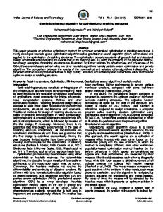
Thus  s (t ) was the probability for solver s  S that a performance ratio rp ,s was within a factor t  R of the best possible ration. Then function  s was the (cumulative) distribution function for the performance ratio. The performance profile  s : R  [0, 1] for a solver was a nondecreasing, piecewise constant function, continuous from the right at each breakpoint. The value of  s (1) was the probability that the solver would win over the rest of the solvers. According to the above rules, we know that one solver whose performance profile plot is on top right will win over the rest of the solvers. In Figures 1-3, NA denotes Algorithm 1, PRP denotes Algorithm 2, and PRP+ denotes Algorithm 3. Figures 1-3 show that the performance of these methods is relative to NT  NF  m  NG , where NF and NG denote the number of function evaluations and gradient evaluations respectively, and m is an integer. According to the results on automatic differentiation [30], the value of m can be set to m  5 . That is to say, one gradient evaluation is equivalent to m number of function evaluations if automatic differentiation is used. From these three figures Copyright © 2010 SciRes.

Figure 2. Performance profiles(NT) of methods with strong Wolfe-Powell rule

Figure 3. Performance profiles (NT) of methods with weak Wolfe-Power rule JSEA


508

it is clear that the given method has the most wins (has the highest probability of being the optimal solver). In summary, the presented numerical results reveal that the new method, compared with the normal PRP method and the modified PRP method [14], has potential advantages.

5. Conclusions This paper gives a new line search method for unconstrained optimization. The global and R-linear convergence are established under weaker assumptions on the search direction d k . Especially, the direction d k satisfies the sufficient condition (5) and the condition (9) without carrying out any line search technique, and some paper [14,27,30] often obtains these two conditions by assumption. The comparison of the numerical results shows that the new search direction of the new algorithm is a good search direction at every iteration.

REFERENCES

with a Strong Global Convergence Properties,” SIAM Journal of Optimization, Vol. 10, No. 1, 2000, pp. 177182. [12] Z. Wei, G. Li, and L. Qi, “New Nonlinear Conjugate Gradient Formulas for Large-Scale Unconstrained Optimization Problems,” Applied Mathematics and Computation, Vol. 179, No. 2, 2006, pp. 407-430. [13] G. Yuan and X. Lu, “A Modified PRP Conjugate Gradient Method,” Annals of Operations Research, Vol. 166, No. 1, 2009, pp. 73-90. [14] J. C. Gibert, J. Nocedal, “Global Convergence Properties of Conjugate Gradient Methods for Optimization,” SIAM Journal on Optimization, Vol. 2, No. 1, 1992, pp. 21-42. [15] Y. Dai and Y. Yuan, “Nonlinear Conjugate Gradient Methods,” Shanghai Science and Technology Press, 2000. [16] E. Polak and G. Ribiè, “Note Sur la Xonvergence de Directions Conjugèes,” Rev Francaise Informat Recherche Operatinelle 3e Annèe, Vol. 16, 1969, pp. 35-43. [17] M. J. D. Powell, “Nonconvex Minimization Calculations and the Conjugate Gradient Method,” Lecture Notes in Mathematics, Springer-Verlag, Berlin, Vol. 1066, 1984, pp. 122-141.

[1]

G. Yuan and X. Lu, “A New Line Search Method with Trust Region for Unconstrained Optimization,” Communications on Applied Nonlinear Analysis, Vol. 15, No. 1, 2008, pp. 35-49.

[2]

G. Yuan, X. Lu, and Z. Wei, “New Two-Point Stepsize Gradient Methods for Solving Unconstrained Optimization Problems,” Natural Science Journal of Xiangtan University, Vol. 29, No. 1, 2007, pp. 13-15.

[19] W. W. Hager and H. Zhang, “A New Conjugate Gradient Method with Guaranteed Descent and an Efficient Line Search,” SIAM Journal on Optimization, Vol. 16, No. 1, 2005, pp. 170-192.

[3] G. Yuan and Z. Wei, “New Line Search Methods for Uncons- trained Optimization,” Journal of the Korean Statistical Society, Vol. 38, No. 1, 2009, pp. 29-39.

[20] Z. Wei, S. Yao, and L. Liu, “The Convergence Properties of Some New Conjugate Gradient Methods,” Applied Mathematics and Computation, Vol. 183, No. 2, 2006, pp. 1341-1350.

[4]

Y. Yuan and W. Sun, “Theory and Methods of Optimization,” Science Press of China, Beijing, 1999.

[5]

D. C. Luenerger, “Linear and Nonlinear Programming,” 2nd Edition, Addition Wesley, Reading, MA, 1989.

[6]

J. Nocedal and S. J. Wright, “Numerical Optimization,” Springer, Berlin, Heidelberg, New York, 1999.

[7]

Z. Wei, G. Li, and L. Qi, “New Quasi-Newton Methods for Unconstrained Optimization Problems,” Applied Mathematics and Computation, Vol. 175, No. 1, 2006, pp. 11561188.

[8]

Z. Wei, G. Yu, G. Yuan, and Z. Lian, “The Superlinear Convergence of a Modified BFGS-type Method for Unconstrained Optimization,” Computational Optimization and Applications, Vol. 29, No. 3, 2004, pp. 315-332.

[9] G. Yuan and Z. Wei, “The Superlinear Convergence Analysis of a Nonmonotone BFGS Algorithm on Convex Objective Functions,” Acta Mathematica Sinica, English Series, Vol. 24, No. 1, 2008, pp. 35-42. [10] G. Yuan and Z. Wei, “Convergence Analysis of a Modified BFGS Method on Convex Minimizations,” Computational Optimization and Applications, Science Citation Index, 2008. [11] Y. Dai and Y. Yuan, “A Nonlinear Conjugate Gradient


[18] L. Grippo and S. Lucidi, “A Globally Convergent Version of the Polak-RibiÈRe Gradient Method,” Mathematical Programming, Vol. 78, No. 3, 1997, pp. 375-391.

[21] G. H. Yu, “Nonlinear Self-Scaling Conjugate Gradient Methods for Large-scale Optimization Problems,” Thesis of Doctor's Degree, Sun Yat-Sen University, 2007. [22] G. Yuan, “Modified Nonlinear Conjugate Gradient Methods with Sufficient Descent Property for Large-Scale Optimization Problems,” Optimization Letters, Vol. 3, No. 1, 2009, pp. 11-21. [23] G. Yuan, “A Conjugate Gradient Method for Unconstrained Optimization Problems,” International Journal of Mathematics and Mathematical Sciences, Vol. 2009, 2009, pp. 1-14. [24] G. Yuan, X. Lu, and Z. Wei, “A Conjugate Gradient Method with Descent Direction for Unconstrained Optimization,” Journal of Computational and Applied Mathematics, Vol. 233, No. 2, 2009, pp. 519-530. [25] L. Zhang, W. Zhou, and D. Li, “A Descent Modified Polak-RibiÈRe-Polyak Conjugate Method and its Global Convergence,” IMA Journal on Numerical Analysis, Vol. 26, No. 4, 2006, pp. 629-649. [26] Y. Liu and C. Storey, “Efficient Generalized Conjugate Gradient Algorithms, Part 1: Theory,” Journal of Optimization Theory and Application, Vol. 69, No. 1, 1992, pp. 17-41.

JSEA


509

[27] Z. J. Shi, “Convergence of Line Search Methods for Unconstrained Optimization,” Applied Mathematics and Computation, Vol. 157, No. 2, 2004, pp. 393-405.

[29] E. D. Dolan and J. J. Moré, “Benchmarking Optimization Software with Performance Profiles,” Mathematical Programming, Vol. 91, No. 2, 2002, pp. 201-213.

[28] J. J. Moré, B. S. Garbow, and K. E. Hillstrome, “Testing Unconstrained Optimization Software,” ACM Transactions on Mathematical Software, Vol. 7, No. 1, 1981, pp. 17-41.

[30] Y. Dai and Q. Ni, “Testing Different Conjugate Gradient Methods for Large-scale Unconstrained Optimization,” Journal of Computational Mathematics, Vol. 21, No. 3, 2003, pp. 311-320.


JSEA