International Journal of
Geo-Information Article
A Local Land Use Competition Cellular Automata Model and Its Application Jun Yang 1,2, *, Junru Su 1 , Fei Chen 1 , Peng Xie 3 and Quansheng Ge 2 1 2 3
*
Liaoning Key Laboratory of Physical Geography and Geomatics, Liaoning Normal University, Dalian 116029, China;
[email protected] (J.S.);
[email protected] (F.C.) Key Laboatory of Land Surface Pattern and Simulation, Institute of Geographic Sciences and Natural Resources Research, CAS, Beijing 100101, China;
[email protected] School of Resource and Environmental Sciences, Wuhan University, Wuhan 430079, China;
[email protected] Correspondence:
[email protected]; Tel.: +86-411-8215-9237
Academic Editors: Qiming Zhou, Zhilin Li and Wolfgang Kainz Received: 14 April 2016; Accepted: 27 June 2016; Published: 30 June 2016
Abstract: Cellular automaton (CA) is an important method in land use and cover change studies, however, the majority of research focuses on the discovery of macroscopic factors affecting LUCC, which results in ignoring the local effects within the neighborhoods. This paper introduces a Local Land Use Competition Cellular Automata (LLUC-CA) model, based on local land use competition, land suitability evaluation, demand analysis of the different land use types, and multi-target land use competition allocation algorithm to simulate land use change at a micro level. The model is applied to simulate land use changes at Jinshitan National Tourist Holiday Resort from 1988 to 2012. The results show that the simulation accuracies were 64.46%, 77.21%, 85.30% and 99.14% for the agricultural land, construction land, forestland and water, respectively. In addition, comparing the simulation results of the LLUC-CA and CA-Markov model with the real land use data, their overall spatial accuracies were found to be 88.74% and 86.82%, respectively. In conclusion, the results from this study indicated that the model was an acceptable method for the simulation of large-scale land use changes, and the approach used here is applicable to analyzing the land use change driven forces and assist in decision-making. Keywords: local land use competition; cellular automata; land simulation; Jinshitan National Tourist Holiday Resort
1. Introduction Land resources are the most fundamental and important resources in human life and production. They are not only related to the structure and function of ecosystems, but also affect the global interaction between the ecosystems and land surface environment [1]. Different land use types have different social, economic, environmental, and ecological development functions, and exist in a state of dynamic equilibrium. Land use change is a complex process caused by the interactions between nature and social systems at several spatial and temporal scales [2,3]. The diverse demand of society for limited land resources is the root of land use competition occurrences, and in essence it is a type of competing interest, which eventually creates mutual conversions between land use types [4]. Dynamic changes in land resources are embodied in the competitive process between the various types of land use. It is a process that maximizes the satisfaction of the new demand of the land use by weighing and changing the land use patterns following the changes of the human demand for the land use [5]. Models characterized by simplifying and abstracting play a very important role in understanding and predicting the patterns and evolution process of LUCC. Currently, there are many valuable land ISPRS Int. J. Geo-Inf. 2016, 5, 106; doi:10.3390/ijgi5070106
www.mdpi.com/journal/ijgi
ISPRS Int. J. Geo-Inf. 2016, 5, 106
2 of 15
use change simulation and prediction models and related research work, which typically include the system dynamics model (SD) [6], Markov model [7], conversion of land use and its effects at small regional extent (CLUE-S) model, multi-agent systems (MAS) model [8,9], cellular automata (CA) model [10–13], and the integration of these models [14]. Many studies emphasize in particular a macro perspective of the driving factors to simulate land use changes. However, in fact, land use changes are often the results of the integrated effects of the natural and human macroscopic and microscopic factors. The question remains as to how to begin from the point of view of the micros of local land use competition, and then combine the macro driving factors and the micro effects for the purpose of building a reliable land use change simulation model, which has currently become a breakthrough worthy of studying. Miller suggests that relationships among near entities do not signify a simple and sterile geography, and complex geographic processes and structures can emerge from local interactions [15]. CA is a grid dynamics model, in which time, space, and state are all discrete, and the spatial interaction and temporal causality are both local. This model has been able to simulate the spatiotemporal evolution process of complicated systems [16–19]. The state of each cell changes over time, and is determined by the local transition rules, where a large number of cells comprise the evolution of the dynamic systems through simple interaction [20]. Wolfram proved that a CA model could simulate the complex natural phenomena, and the local behavior between individuals can evolve the global change patterns in time and space [21]. Recently, CA models have been increasingly applied in the simulation and prediction of urban expansion and land use change research, and have obtained significant results, which indicate that a CA model can effectively reflect the complex features of land use evolution at the microscopic pattern [22–25]. It is a basic feature of a CA that global dynamic behavior can evolve from local rules. In land use models, CA can typically model the transition of a cell from one land use to another, depending on the land use within the neighborhood of the cell [26]. Spatial variations in the relationships between driving forces and land use change are ignored in conventional land use CA models, which are based on assumption of spatial homogeneity [27]. The existing CA models greatly weakened the fundamental characteristics of the original scheme of CA with the introduction of intelligent methods, and the continuous relaxation of the model constraints [28]. The majority of the previous studies have focused on constraint design, influencing factors, and their intelligent acquisition, in order to improve the CA simulation results from a macro perspective. However, one of the most important characteristics of a CA is the local effect within a neighborhood. The lack of research on local effects and principles has lost the advantage of global change simulation through local interaction. One important method of solving this problem is to pay more attention to the study of the spatial relationship of the local scale, while introducing a number of macro geographical restrictions to the CA. Yang et al., (2014) designed a land use change simulation CA model, which focused on the cell type of land use conversion in multiple directions, and indicated that the transition probability of each cell could be influenced by not only the same land use cells, but also the different land use cells [29]. Sirakoulis et al., (2012) designed a CA model based on an irregular neighborhood, which reflected a very good consideration of local interaction, and the transition potential for the cell could be defined by using the intensities of the signals received from the other cells within the neighborhood [30]. Land use change study not only requires both global and macro-scales, but also needs local and micro-scale to be cooperative [31,32]. CA provides the spatial-temporal dynamic simulation computing framework by using a bottom-up approach, and it can achieve a land use change simulation under the comprehensive impact of macroscopic natural and social factors, as well as the interaction of the local neighborhood of cells [33–35]. Based on the achievements listed above, in this study, a Local Land Use Competition Cellular Automata (LLUC-CA) model is introduced, which is based on local land use competition, land suitability evaluations, demand analysis of the different land use types, and a multi-target land use competition allocation algorithm, for the purpose of simulating the land use changes at a micro level, which focuses on the understanding of the neighborhood effects in the
ISPRS Int. J. Geo-Inf. 2016, 5, 106
3 of 15
ISPRS Int. J. Geo-Inf. 2016, 5, 106
15 simulating the land use changes at a micro level, which focuses on the understanding of3 ofthe neighborhood effects in the simulation process. In order to discuss the land use change simulation method based on aInLLUC-CA, and to the change reliability of the model, wellon asa to provide simulation process. order to discuss theverify land use simulation methodas based LLUC-CA, theoretical and for theas simulation prediction of land changes, a casefor study and to verify thetechnical reliabilitysupport of the model, well as toand provide theoretical anduse technical support the was conducted at the Jinshitan National Tourist Holiday Resort (hereinafter referred to as Jinshitan), simulation and prediction of land use changes, a case study was conducted at the Jinshitan National which isHoliday a very local extent. Tourist Resort (hereinafter referred to as Jinshitan), which is a very local extent.
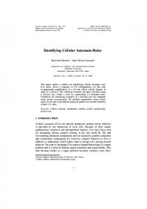
2. Data Dataand andMethods Methods 2.1. Study Area ˝ 81 102 N, Jinshitan, the theback back garden of Dalian, Liaoning China (39˝ 11 492 –39 garden of Dalian, Liaoning Province,Province, China (39°1′49″–39°8′10″N, 121°56′11″– is located in Peninsula the Liaodong in the area 1). of It Dalian 122°4′42″E), is located in the Liaodong in thePeninsula northeastern areanortheastern of Dalian (Figure faces (Figure 1). It faces the Yellow Sea on the east, and is composed of the eastern peninsula, western the Yellow Sea on the east, and is composed of the eastern peninsula, western peninsula, open peninsula, open and the between the two peninsulas. It approximately covers a land 58 area heartland, and theheartland, beach between thebeach two peninsulas. It covers a land area of kmof2. 2 approximately 58 km . Located to the Dalian urban area, it isa arural–urban typical area zone with aand rural–urban Located adjacent to the Dalian adjacent urban area, it is a typical area with a coastal zone and a coastal region. Beginning as a rural town dominated by traditional agriculture, it was region. Beginning as a rural town dominated by traditional agriculture, it was identified as a National identified asina 1988, National ScenicGeopark Spot in 1988, National Geopark of Tourist China inArea 2004,inand a 5A Tourist Area Scenic Spot National of China in 2004, and a 5A 2010. Its construction in 2010. Its construction and development into a tourist resort in China had a strong representation. and development into a tourist resort in China had a strong representation. For nearly 25 years, the For nearly years, the study area haseconomic experienced rapid economic and land change, study area25has experienced rapid development and development land use change, anduse therefore and therefore research value. possesses highpossesses research high value.
121˝ 561 112 –122˝ 41 422 E),
Figure 1. 1. Location Location of of study study area, area, Dalian, Dalian, Liaoning, Liaoning, China. China. The The remote remote sensing sensing image image was was generated generated Figure based on on 10 10 m m multispectral multispectral and and 2.5 2.5 m m panchromatic panchromatic spatial spatial resolution resolution SPOT5 SPOT5 image. image. based
2.2. Data Sources and and Processing Processing 2.2. Data Sources The years years 1988, 1988, 2004 2004 and and 2010 2010 are are three three time time nodes nodes that that have have important important significance significance to to the the The development of Jinshitan. In view of the data accessibility, this study based its research on the land development of Jinshitan. In view of the data accessibility, this study based its research on the land use data data of of 1988, 1988, 2003 2003 and and 2012. 2012. The map use The real real land land use use maps maps were were mainly mainly obtained obtained from from the the 1:10,000 1:10,000 map scale vector land use database. The administrative map, road, town center and coastline data were scale vector land use database. The administrative map, road, town center and coastline data were mainly obtained obtained from from the the comprehensive comprehensive underlying underlying database. database. All were provided provided by by mainly All of of these these data data were
ISPRS Int. J. Geo-Inf. 2016, 5, 106
4 of 15
the Dalian Municipal Bureau of Land Resources and Housing, including the topographic maps and remote sensing images. By combining the land use vector data with the high spatial resolution remote sensing images, the respective maps of land use of Jinshitan in 1988, 2003 and 2012 were acquired by a series of processing, such as projection transformation, spatial adjustment, topology error checks, cutting, image interpretation, and data normalization. ArcGIS10.2 and ERDAS Imaging 2013 software were used. In order to simplify simulation process, the land use types were reclassified into agriculture land, construction land, forestland, and water by ArcGIS. The first three land use types obtained a large proportion and changed more obviously, and water was an important natural resource that had an outstanding effect on Jinshitan (Table 1). All of the spatial data were standardized to the Xi’an 80 geographic coordinate system and Gauss Kruger zone dividing projected coordinate system, and the raster data was resampled with a grid size of 5 m ˆ 5 m. Table 1. Classification of land use types. Land Use Type
Code
Meaning
Agricultural land
A
Refers to land directly used for agricultural production, including cultivated land, garden land, grassland and other farmland
Construction land
C
Refers to the land used for construction of the buildings and structures, including land for scenic and recreation facilities, commercial service, industry, mining, warehouse, residential, public management, public service, transportation, special demands, etc.
Forestland
F
Refers to untapped forests, weeds, land less disturbed by human activity, and other land except agricultural and construction land
Water
W
Refers to the water surface of rivers, lakes and reservoirs, tidal flat swamps, etc.
2.3. The Model Through local interactions, a CA can simulate global changes, while the global computing capacity is achieved by local computation. In global models, it is assumed that all variables are the same. However, one possible situation is that global models cannot be expressed very effectively in a specific location. Therefore, an LLUC-CA model uses cells in different land use types within a neighborhood as the neighborhood scenario, and forms local transition rules through the combination of the local land use competition and the macro driving factors. With these rules in place, it can evolve the global and complex dynamic behavior, and then simulate all of the land use changes. 2.3.1. Local Land Use Competition At the present time, the land use science community has not yet clearly defined the meaning of local land use competition. Before further research is conducted, a clear definition should be made regarding this scientific question. In physical geography, the term “local” may be some area over which a particular process has an obvious effect. However, in terms of spatial data analysis, a “local space” is often expressed as a certain distance of space starting from a specific point or an area, for example, the locality or neighborhood of that point or area [36]. Local interactions among entities are capable of generating complex global behaviors, as well as intricate structures in space and time [15]. In this study, “local land use competition (LLUC)” is defined as a mutual competition between the different land use types in the neighboring regions. Local land use competition materializes as the mutual competition between the different state of cellular within a neighborhood, with the interaction intensity of the cell decreasing with the increase of the distance between the cells, and the scope of the workspace embodied in the locality. Therefore, the competition result is the land use state change of the central cell. Land use changes occur due to competition within and among different land use types. Spatial autocorrelation not only acts on the same land use type cells, but also on the different types of land use cells. This study assumed that there were three land use types, namely agricultural land
ISPRS Int. J. Geo-Inf. 2016, 5, 106
5 of 15
(A), construction land (C) and forestland (F), in a 5 ˆ 5 Moore neighborhood (radius r = 2), and the ISPRS Int. J. Geo-Inf. 2016, 5, 106 of 15 different land use type cells were denoted with different colors. Under the effects of local 5land use competition and macro driving factors, the cells in a certain state can transition to multiple directions, competing relationship between the land use types is illustrated with Figure 2. As shown in the andfigure, the competing relationship between the land use types is illustrated with Figure 2. As shown in Num (A) = 7 expressed that the number of cells of the agricultural land in the neighborhood the figure, Num (A) 7 expressed thatthat thethe number ofof cells agricultural land in the neighborhood scenario is 7, Num=(C) = 8 expressed number cellsofofthe construction land in the neighborhood scenario is 7,isNum expressed thatthat thethe number of cells of construction in the scenario 8, and(C) so = on.8 Due to the fact land type transformation of theland central cell neighborhood was based scenario is 8, and so on. Due to the fact that the land type transformation of the central cell wasnot based on its independent neighborhood scenario, the interactions between the land use types were on its independent neighborhood scenario, the interactions between the land use types were not equal. equal.
Figure 2. Sketch mutualcompetition competition between between different cells in the neighborhood. Figure 2. Sketch of of mutual differentland landuse usetype type cells in the neighborhood.
The competition relationship between the central and neighbor cells is expressed by the land use The competition relationship between the central and neighbor cells is expressed by the land use competition intensity. The land use competition intensity was constantly changing, it was a dynamic competition intensity. land use intensity was and constantly changing, was a dynamic parameter, and wasThe inspired by competition spatial interaction model, the local land useit competition parameter, was inspired by spatial model, thetlocal land use competition intensity intensityand of the cell (i,j), which state (orinteraction land use type) is k,and at time can be described as:
of the cell (i,j), which state (or land use2 type) is k, at time t can be described as: 2 [ J s t (i x, j y ) / d (i x, j y )] 2 2 (1) ` ˘ 2 řx 2 yř Ckt i, j rJ st pi ` x,Nj ` yq {dpi ` x, j ` yqs x“´2 y“´2 Ckt pi, jq “ (1) where N is the total number of cells in the central N cell’s neighborhood (in this study it is 25); J(St(i+x,j+y)) is used for judging the state of cell (i+x,j+y), whether it is k, 1 for true, and 0 for false;
t (i+x,j+y)) where N is theistotal number ofkernel, cells inand the central cell’s neighborhood thisthe study it is 25); d(i+x,j+y) convolution it represents the distance (in from central cellJ(S(i,j) to is used for judging the state of cell (i+x,j+y), whether it is k, 1 for true, and 0 for false; d(i+x,j+y) neighborhood cell (i+x,j+y), if (i+x,j+y) is the central cell, d(i+x,j+y)=1; otherwise if (i+x,j+y) is just close is convolution kernel, and it or represents from the central cell then (i,j) to neighborhood to (i,j), then d(i+x,j+y)=2; if (i+x,j+y)the anddistance (i,j) are separated by one cell, d(i+x,j+y)=3. If the cell (i+x,j+y), if (i+x,j+y) the central cell, d(i+x,j+y)=1; otherwise neighborhood cell is closer to the central cell, the impact on it willifbe(i+x,j+y) greater. is just close to (i,j), then d(i+x,j+y)=2; or if (i+x,j+y) and (i,j) are separated by one cell, then d(i+x,j+y)=3. If the neighborhood Land and Transition Potential cell 2.3.2. is closer toSuitability the central cell, the impact on it will be greater.
ISPRS Int. J. Geo-Inf. 2016, 5, 106
6 of 15
2.3.2. Land Suitability and Transition Potential The process of LUCC is very complex, and the suitability conditions play a very important role in the land use transition, in addition to the local neighborhood effect. In order to make the land suitability analysis feasible both biophysically and socioeconomically, a comprehensive consideration of the social, economic, political, environmental, and other driving factors, as well as a reflection of the different influences of these factors are needed. Therefore, in this model a series of suitability index layers LK pi, jq for each type of land use was built using the method of multi-criteria evaluation (MCE): Lk pi, jq “
α ´ ÿ m “1
Fk, f ˆ Wk, f
β ¯ź
Fk, f
(2)
m “1
where Fk,f refers to the scoring of criteria f to land type k, and this score is normalized to 0~1 by the maximum value method. When 1 ő m ő α, Fk,f indicates that the factors composed of a group of spatial distance variables and topography. When 1 ő m ő β, Fk,f indicates the constraints composed by protected land, topography, and so forth, and the value of this score is 1 or 0. The weight of factor f for land use type k is represented by Wk,f , and was acquired by an AHP method [37]. Each cell corresponded to a certain type of land use. The historical trends of the land use changes, land suitability, and related policies and economics were used to construct the transition rules. They controlled the transition possibility of each cell together, and the state of the cell changed when its probability exceeded the control threshold. The cells within the cellular space synchronize update state according to these local transition rules, and the entire cellular space was shown as the change in the discrete time dimension. The definition of the transition rules is the simulate core part of a standard CA, and they can guide a dynamic evolution. The LLUC-CA model’s transition rules can be indicated as the land use transition potential. Due to the complexity of nature, some unforeseen characteristics of the process of land use change cannot be explained by independent variables. This can cause the simulation results to be closer to reality through the introduction of random variable to express the uncertainty of the nature and geography of a CA. In each simulation, the final transition probabilities to land use k of cell (i,j) at time t were calculated by the local land use competition intensity, land suitability index, and random variable as follows: ` ˘ ptk pi, jq “ Ckt pi, jq ˆ Lk pi, jq ˆ 1 ` p´lnγqα
(3)
where γ is a random variable with a range from 0 to 1, and α is a parameter for the control of the random variable range. The dynamic iterative calculation of the neighborhood change is required in the land use change simulation process, the neighborhood cell state is dynamic, so that the land use transition potential is also dynamic, and at each time step the transition rules of the model are updated. 2.3.3. Demand Analysis of Different Land Types Aside from the competition between the different land use types and the land suitability, the land use change pattern also depended on the demand for the land use. The Markov model, as a raster-based spatial probability model, is often used to forecast geographical events that have no after-effect characteristics, and has been widely applied to LUCC simulations. Under the assumption that the current social economic mode is under the condition of constant development, the Markov model has the capacity to predict the quantity change of the land use types in the future [38,39]. The transition areas file from a Markov Chain analysis of two prior land use maps established the quantity of the expected land use change from each existing category to each other category during the next time period. Assuming that there are m kinds of land use types, from time t to time t+1 the land use state i transform to j(i,j = 1, 2, ..., m), then the transition probability can be described as:
ISPRS Int. J. Geo-Inf. 2016, 5, 106
7 of 15
Pij “
∆Aij
(4)
Ait
where At i is the area of land use type i at time t, and ∆Aij is the changed area from time t to time t+1 , then the land use state i transform to j. Since there are m kinds of possible states during the land use change process, the transition probability matrix is represented as follows: » — ` ˘ — P “ Pij “ — — –
where 0 ő Pij ő 1 and
řm
j“1 Pij
P11 P21 .. . Pm1
P12 P22 .. . Pm2
¨¨¨ ¨¨¨ .. . ¨¨¨
fi P1m ffi P2m ffi ffi ffi fl Pmm
(5)
“ 1. Therefore, at time t + 1, the area of land use type k can be described as: Akt`1 “
m ÿ `
Ait ˆ Pik
˘
(6)
i “1
2.3.4. Multi-Target Land Use Competition Allocation Algorithm The land use transition potential determined the possible location and direction of the land use state change. The different types of land use demands determined the quantity of the land use changes, and the two worked together to determine the final land use pattern. In most models, a rule-based system is used to allocate the actual land use changes based on the suitability map, including using a threshold to select the locations with the highest suitability, or simulate the land use competition based on the land use type specific characteristics [26]. Assuming that there are m kinds of land use types, from Figure 3 and Equation (3) it can be determined that there are m kinds of transition possibilities and corresponding potentials for cell (i,j) at time t. A simple method is to compare the m transition potentials, and the land use types with the highest potential as the land use change direction for cell (i,j). However, this will lead to the explosion phenomenon of the dominant land use type. In this study, a multi-target land use competition allocation algorithm was built, with the land use transition potential as the basis, and the land use demand as a constraint. It was able to meet the demands of the different land use types on the spatial locations and quantities in the process of the simulation. The algorithm was an allocation mechanism based on a variety of land categories as the initial simulation, which could simulate the multiple land use changes. In Figure 3, the flow chart of the multi-target land use competition allocation algorithm can be seen, which was divided into four steps: (1) Search the cell which has the maximum value of transition potential as Maxpptk pi, jqq of the land use map, keep a record of the position (i,j) and the land use change direction k; (2) Compute the area of land use type k as Atk ; (3) Compare Atk and the area of land use demand Atk`1 predicted by Markov model, if Atk is exceed or equal to Atk`1 , go to step four; otherwise change the land use state St pi, jq of cell (i,j) to k, set the potential pt pi, jq of cell (i,j) as zero, discard the other potential of cell (i,j), then go back to step one; (4) If all kinds of land use types demands are satisfied, or all the cells are changed, then stop the allocation, we will acquire the simulated land use map at time t+1; otherwise, we set all cells’ transition potential Pkt to land use k as zero, give up the possibility of other cells transform to land use k, then go back to step one. 2.3.5. LLUC-CA Model Structure Figure 4 is the model structure of the local land use competition cellular automata (LLUC-CA). The CA was combined with the Markov model to control the transition quantity when coupled with the GIS, and the local rules were used to simulate the global and complex patterns of the land use. The model adopted a loose structure, and the GIS, MCE, Markov, and CA programs run independently,
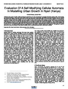
ISPRS Int. J. Geo-Inf. 2016, 5, 106 ISPRS J. Geo-Inf. 5, 106 three Int. stages, as 2016, follows:
8 of 15
15 data preprocessing and input, parameter setting and production,8 of and decision-making of the land use type changes and output. In the first stage, ArcGIS, ERDAS, IDRISI, as well as other software, were used to process the land use map, remote sensing images, topography, exchanging information via data files. The spatial data’s input, conversion, and spatial analysis were and planning data, as well as to create a comprehensive geographic information database, where the performed in the GIS software, the data were extracted from the GIS database, and then input into data structure was consistent, and the spatial reference was unified. In the second stage, the required the MCE, Markov, and CA program for processing. The computation results were then transmitted to parameters for the LLUC-CA were acquired, which included: the land use competition intensity the GIS for display and further processing. The LLUC-CA model consisted of three stages, as follows: index under the influence of local land use competition at the scale of a cellular neighborhood; the data preprocessing and input, parameter setting and production, and decision-making of the land use land suitability index computed by MCE under the influence of land use macro driving factors; and type changes and output. In the first stage, ArcGIS, ERDAS, IDRISI, as well as other software, were the area demand for the different land use types predicted by the Markov model. In the last stage, used to process the land use map, remote sensing images, topography, and planning data, as well as to based on the land use transition potential, which was computed by the local land use competition create a comprehensive geographic information database, where the data structure was consistent, intensity, land suitability and random variables, and different land use area restriction demands, and the spatial reference was unified. In the second stage, the required parameters for the LLUC-CA every cell’s land use type change was determined with a multi-target land use competition allocation were acquired, which included: the land use competition intensity index under the influence of local algorithm. The prototype of the LLUC-CA was implemented in Visual Studio 2010 integrated land use competition at the scale of a cellular neighborhood; the land suitability index computed by development environment, and the program language was Python. The GDAL and Numpy library MCE under the influence of land use macro driving factors; and the area demand for the different land functions were also used. use types predicted by the Markov model. In the last stage, based on the land use transition potential, which was computed by the local land use competition intensity, land suitability and random variables, 2.4. Model Parameters Prepare and Implementation and different land use area restriction demands, every cell’s land use type change was determined addition to the of the actual land use, the following parameters also needed to be with In a multi-target landbasic use map competition allocation algorithm. The prototype of the LLUC-CA was prepared in order to implement theintegrated LLUC-CAdevelopment model in theenvironment, study area: the computation the land implemented in Visual Studio 2010 and the programoflanguage suitability maps theNumpy MCE method, and the computation of the transition matrix using the was Python. The based GDALon and library functions were also used. Markov chain analysis.
Figure 3. 3. Flow of multi-target multi-target land land use use competition competition allocation allocation algorithm. algorithm. Figure Flow chart chart of
ISPRS Int. J. Geo-Inf. 2016, 5, 106 ISPRS Int. J. Geo-Inf. 2016, 5, 106
9 of 15
9 of 15
Figure the LLUC-CA. LLUC-CA. Figure4.4.Model Model structure structure of the
ThisParameters study considered the Implementation effects of the current land use situation, town centers, main roads, 2.4. Model Prepare and light rail, coastline, and the topographic and spatial regulation of the construction land, based on the In addition the basic mapcharacteristics, of the actual land parameters also to be biophysical andtosocioeconomic on theuse, landthe usefollowing changes, for the purpose of needed computing prepared in order to implement the LLUC-CA model in the study area: the computation of the land the suitability maps for the agricultural land, construction land, forestland, and water, respectively. suitability maps based on the MCE method, and the computation of the transition matrix using Among these, the scores of the first five factors to the four land use types were evaluated by distance,the Markov chain analysis. the topographic data were expressed by slope, and the results were standardized (values between 0 This considered the effects the25% current use situation, town centers, main roads, and 1). study The areas with a slope greater of than were land not allowed for cultivation and construction, light rail, coastline, and the topographic and spatial regulation of the construction land, based on the the transportation land was not suitable for cultivation, and the spatial regulation of the construction land did and not allow construction. These threeon criteria were constraints forpurpose the landofsuitability biophysical socioeconomic characteristics, the land usethe changes, for the computing integrated combining domain experts the AHPand method was adopted theevaluation. suitabilityAn maps for themethod agricultural land, the construction land, and forestland, water, respectively. to obtain the relative significance values of the factors contributing to the suitability of the for Among these, the scores of the first five factors to the four land use types were evaluated byland distance, development. A satisfactory Consistency Ratio was obtained for the four land use types (Table 2). 0 the topographic data were expressed by slope, and the results were standardized (values between to Equation (3), and standardized images, the mapsthe andSubsequently, 1). The areasaccording with a slope greater than 25% the were not allowedcriteria for cultivation andsuitability construction, for 2003 were calculated using the MCE method (Figure 5). transportation land was not suitable for cultivation, and the spatial regulation of the construction land did not allow construction. These three criteria were the constraints for the land suitability evaluation. Table 2. Weights of influencing factors of land suitability. An integrated method combining the domain experts and the AHP method was adopted to obtain the relative significance values of the factors contributing to theWeights suitability of the land for development. Factors A fourCland use F typesW(Table 2). Subsequently, A satisfactory Consistency Ratio was obtained for the Distance to town center 0.0915 0.2562 0.0255 0.0428 according to Equation (3), and the standardized criteria images, the suitability maps for 2003 were Distance to light rail 0.0723 0.1513 0.0573 0.0275 calculated using the MCE method (Figure 5).
Distance to water Distance to forestland Distance to construction land Distance to agricultural land Slope ISPRS Int. J. Geo-Inf. 2016, 5, 106 Consistency Ratio
0.1732 0.0754 0.1576 0.1739 0.0413 0.0512
0.0303 0.0379 0.1622 0.0528 0.0340 0.0427
0.1363 0.3035 0.0396 0.0860 0.2546 0.0498
0.3315 0.0573 0.0987 0.1098 0.0436 0.0787
10 of 15
Figure 5.5.Suitability (b) construction constructionland; land;(c) (c)forestland; forestland;and and(d) (d) water. Figure Suitabilitymaps mapsfor: for:(a) (a)agricultural agricultural land; (b) water. Table 2. was Weights of to influencing of land suitability. The Markov chain analysis used computefactors the transition probabilities matrix based on the actual land use maps from 1988 to 2003, and then Equation (6) was used to compute the different Weights land use types demand forFactors 2012 (Table 3). A C F W Table 3. Land use transition probability matrix and area demand. Distance to town center 0.0915 0.2562 0.0255 0.0428 Distance to light rail 0.0723 0.1513 0.0573 0.0275 For 2012 0.0717 Distance to main road 0.1830 0.2277 0.0412 Land Use Type Distance to coastline 0.0318 0.0476 0.0255 0.2476 A C F W Distance to water 0.1732 0.0303 0.1363 0.3315 Distance to forestland A 0.0754 0.3787 0.03790.12710.3035 0.4937 0.0005 0.0573 Distance to construction land 0.1576 0.1622 0.0396 0.0987 C 0.0331 0.8706 0.0943 0.0020 Distance to agricultural land 0.1739 0.0528 0.0860 0.1098 From 2003 Slope 0.0413 0.1574 0.03400.82310.2546 F 0.0185 0.0010 0.0436 Consistency Ratio 0.0512 0.0427 0.0498 0.0787 W 0.0103 0.0861 0.0456 0.8581
Land demand (km2)
5.5555
23.6500
23.7525
4.9942
The Markov chain analysis was used to compute the transition probabilities matrix based on the actual land use maps from 1988 to 2003, and then Equation (6) was used to compute the different land Three datasets ( (1) the 2003 actual land use map; (2) the 2003 land suitability maps; and (3) the use types demand for 2012 (Table 3). demand area for 2012) were input into the LLUC-CA model before running the program. After all the required basic parameters were calibrated (About the details of the model calibration, please see Table 3. Land use transition probability matrix and area demand. reference [40]) and configured, the LLUC-CA simulation program was begun. During the simulation process, the program first produced the local land useForcompetition intensity index, and then 2012 Use Type generated the land useLand transition potential for every cell, which had been integrated with the land A C F W suitability index by Equation (3). The simulated map from 2012 was computed by the multi-target A 0.4937 0.3787 0.1271 0.0005 land use competition allocation algorithm, according to the land use demands. From 2003
3. Results and Discussion
C F W
Land demand (km2 )
0.0331 0.0185 0.0103
0.8706 0.1574 0.0861
0.0943 0.8231 0.0456
0.0020 0.0010 0.8581
5.5555
23.6500
23.7525
4.9942
Three datasets ( (1) the 2003 actual land use map; (2) the 2003 land suitability maps; and (3) the demand area for 2012) were input into the LLUC-CA model before running the program. After all the required basic parameters were calibrated (About the details of the model calibration, please see reference [40]) and configured, the LLUC-CA simulation program was begun. During the simulation process, the program first produced the local land use competition intensity index, and then generated
ISPRS Int. J. Geo-Inf. 2016, 5, 106
11 of 15
the land use transition potential for every cell, which had been integrated with the land suitability index by Equation (3). The simulated map from 2012 was computed by the multi-target land use competition allocation algorithm, according to the land use demands. ISPRS Int. J. Geo-Inf. 2016, 5, 106
11 of 15
3. Results and Discussion 3.1. Analysis of Land Use/Cover Changes 3.1. Analysis of Land Use/Cover Changes The land use cover of Jinshitan developed greatly from 1988 to 2012, from the National Scenic land use cover of Jinshitan developed fromArea. 1988 to 2012, fromtrend the National Spot The to the National Geopark, and then to the greatly 5A Tourist The general was theScenic rapid Spot to of theconstruction National Geopark, andthe then to the 5Adecline TouristofArea. The general trend was the rapid growth land, and continuing agricultural land and forestland, with growth of construction land, continuing decline of agricultural and forestland, with water decreasing slightly, and and thenthe leveling off (Figures 6 and 7a–c). It can land be seen from these figures 2 2 water decreasing slightly, and then leveling off (Figures 6 and 7a–c). It can be seen from these figures that the agricultural land area in 1988 was 21.29 km , and had decreased to 8.97 km in 2003, a 57% 2 , and2 had decreased to 8.97 km2 in 2003, a 57% that the agricultural landthen areafurther in 1988decreased was 21.29tokm decrease in 15 years, and 4.08 km in 2012. Meanwhile, the construction land 2, a2four-fold decrease in 15 years,growth, and then further decreased to 4.08 in 2012. increase Meanwhile, construction experienced a rapid from just 3.62 km2 to 18.16 kmkm in 15the years, resulting 2 to 18.16 km2 , a four-fold increase in 15 years, 2 land experienced a rapid growth, from just 3.62 km in a total land area of 27.97 km in 2012. At the same time, the decrease of the forestland was relatively 2 in2 2012. At the same time, the decrease of the forestland resulting in a totalfrom land26.32 areakm of 227.97 kmkm small, decreasing to 20.28 over the 25-year period, and the area of water remained was relatively small, decreasing 26.32 km to 20.28 km2 over thewas 25-year the area stable. The results indicated that from the increase of2the construction land at theperiod, cost ofand a transition of water remained stable. land The results that the increase the transition construction land was in at the from a large agricultural area, asindicated well as some forest area.ofThis is reflected cost of a transition a large agricultural area, as well as somethat forest area. Thisbetransition is probability matrix from in Table 3 from 2003 toland 2012, which indicates there may 37.83% of reflected in the probability matrix in Table 3 from 2003 to 2012, which indicates that there may be agricultural land converted to construction land, and 12.71% will be converted to forestland; 15.74% 37.83% of agricultural land converted to construction 12.71% willwater be converted to forestland; of forestland will be converted to construction land;land, andand 8.61% of the will be converted to 15.74% of forestland converted to construction land; andland 8.61% of the water willto beforestland, converted construction land. Atwill thebe same time, 9.43% of the construction will be converted to construction At the between same time, theuse construction land will be converted to forestland, and the mutual land. conversion the9.43% other of land types is less significant. and the mutual conversion between the other land use types is less significant.
Figure 6. Area of land use classes in the study area. Figure 6. Area of land use classes in the study area.
3.2. Model Validation 3.2. Model Validation For model validation, the actual land use map for 2012 and the LLUC-CA simulated land use map For model validation, the actual land use map for 2012 and the LLUC-CA simulated land use were compared (Figure 7c,d). The overall simulation land use map was very similar to the actual one map were compared (Figure 7c,d). The overall simulation land use map was very similar to the actual by visual comparison, especially in the middle and southern sections of the study area. The simulation one by visual comparison, especially in the middle and southern sections of the study area. The simulation results of the forestland and water were very close to the actual land use map both in spatial layout and quantity, and the actual water area was 5.63 km2, while the simulation area reached 5.32 km2. These results indicated that the model effectively reproduced the area for each land use type in the land use change simulation. The main deviation was located in the northern areas, where
ISPRS Int. J. Geo-Inf. 2016, 5, 106
12 of 15
results of the forestland and water were very close to the actual land use map both in spatial layout and quantity, and the actual water area was 5.63 km2 , while the simulation area reached 5.32 km2 . These results indicated that the model effectively reproduced the area for each land use type in the land use change simulation. The main deviation was located in the northern areas, where the construction ISPRS Int. J. Geo-Inf. 2016, 5, 106 of 15 land of the northwest and northeast areas were scattered around the agricultural land, and the 12 actual agricultural land area was 4.08 km2 , while the simulation area reached 5.56 km2 . Fan et al. (2013) Fan et al. (2013) conducted related research in Jinshitan from the perspective of a tourist land use conducted related research in Jinshitan from the perspective of a tourist land use landscape pattern, landscape pattern, which also had a high consistency with this study from the perspective of land which also had a high consistency with this study from the perspective of land use patterns [41]. use patterns [41].
Figure 7. 7. Land Land use use maps: maps: (a) (a) actual actual land land use use map map in in 1988; 1988; (b) (b) actual actual land land use use map map in in 2003; 2003; (c) (c) actual actual Figure land use map in 2012; (d) LLUC-CA simulated land use map in 2012; and (e) CA-Markov simulated land use map in 2012; (d) LLUC-CA simulated land use map in 2012; and (e) CA-Markov simulated land use use map map in in 2012. 2012. land
the purpose purpose of of further further verifying verifyingthe theimprovement improvementeffects effectsof ofthetheLLUC-CA LLUC-CA model, For the model, a a comparative study was carried using a CA-Markov model, andsuitability the suitability used comparative study was carried outout using a CA-Markov model, and the mapsmaps used were weresame. the same. The simulation results the CA-Markov are shown in Figure 7e, and very similar the The simulation results of theofCA-Markov are shown in Figure 7e, and are are very similar to to those shown Figure However,the theconstruction constructionand andagricultural agriculturalland landsimulation simulation was was found found to those shown in in Figure 7d.7d. However, southwest, where where the the growth growth area was too large and the simulation be poorer in the northeast and southwest, inaccurate. For For the the quantitative quantitative validation validation of of the the model’s model’s accuracy, accuracy, the actual actual land use position was inaccurate. map and the simulated land use map were verified based on a Kappa coefficient. The LLUC-CA’s Kappa coefficients coefficients were 64.46%, 77.21%, 85.30%, 85.30%, and 99.14% for the agricultural land, construction Kappa The overall overall simulation simulation success success was 88.74%, which land and forestland, and water, respectively. respectively. The meant that for most of the spatial locations of the land use types, the LLUC-CA model performed meant simulations,especially especiallyfor forthe thesimulation simulation forestland and water. other hand, correct simulations, ofof thethe forestland and water. On On the the other hand, the the CA-Markov’s Kappa coefficient 61.54%, 74.62%, 85.12%, and 99.13% foragricultural the agricultural CA-Markov’s Kappa coefficient was was 61.54%, 74.62%, 85.12%, and 99.13% for the land, land, construction landforestlands, and forestlands, and water, respectively, andoverall the overall simulation success construction land and and water, respectively, and the simulation success was was 86.82%, which demonstrated that the spatial accuracy of the simulated land use mapthe using the 86.82%, which demonstrated that the spatial accuracy of the simulated land use map using LLUCLLUC-CA was higher thanofthat the CA-Markov model. In conclusion, the LLUC-CA model CA model model was higher than that theof CA-Markov model. In conclusion, the LLUC-CA model can can potentially be used to simulate use cover change a large scale. potentially be used to simulate landland use cover change on aon large scale.
4. Conclusions The LUCC is a giant complex system, and CA is an important tool that is suitable for complex system simulation. On the one hand, in recent years, research has been mainly concentrated on using artificial intelligence methods to obtain transition rules in order to improve the simulation quality. However, artificial intelligence methods belong to the black box model, and it is not easy to determine
ISPRS Int. J. Geo-Inf. 2016, 5, 106
13 of 15
4. Conclusions The LUCC is a giant complex system, and CA is an important tool that is suitable for complex system simulation. On the one hand, in recent years, research has been mainly concentrated on using artificial intelligence methods to obtain transition rules in order to improve the simulation quality. However, artificial intelligence methods belong to the black box model, and it is not easy to determine the rule hidden under the spatial pattern change. On the other hand, in all types of the extended CA models, without using artificial intelligence algorithms, most can only simulate one target land use type, without the ability to multi-target land use simulation at the same time, and the discovery comprehensive analysis of the relationship between the land use types is weak. The existing regional land use models, as well as the related research, are mainly used for the scope of the study area [14], while in this study, the object of study was not only aimed at a small scale area, but also emphasized the research method of the LLUC-CA cell transition rules within the neighborhood. In this study, a new CA model of local land use competition was introduced, which integrated the advantages of the models, on the basis of summarizing previous research for land use change simulation. In order to explore the interaction mechanism between the various land use types, and to meet the needs of more land types comprehensive simulation, a cellular neighborhood was taken as a local unit. The interaction mechanism within a cellular neighborhood was analyzed, and research of the local land use competition analysis method influenced by the conditions of the cell itself, and land use type distribution within the neighborhood were studied. This study focused on researching this new method of using local land use competition to develop the cell transition rules, explored a multi land use type CA model that had clear physical meaning, and established a complete experiment method. In addition, the land use transition potential generated by combining the local land use competition intensity index, which was computed by local land use competition analysis, the land suitability index computed by the MCE method, and random variables and different area demands that were predicted by the Markov model, were integrated by a multi-target land use competition allocation algorithm, followed by implementing the multi-target land use change simulation. The results indicated that the local land use competition could provide a good expression of the spatial autocorrelation, and the Markov chain analysis helped to control the quantity of land use change. The MCE generated suitability maps in order to help control the spatial distribution of the land use change, and the multi-target land use competition allocation algorithm determined the last change location and quantity. The prototype of the model was programmed by Python and GDAL, which has been successfully applied to the land use change simulation of Jinshitan, using land use maps from 1988, 2003, and 2012. When compared with the LLUC-CA simulated map, the CA-Markov simulated map and the actual land use map, the results indicated that the model had a high simulation accuracy. In the simulation, at the same time, the Kappa coefficient was 64.46%, 77.21%, 85.30%, and 99.14% for the agricultural, construction and forestland, and the water, respectively. The proposed model showed a high accuracy of quantity and spatial distribution in the simulation of the land use changes. The model had a strong spatial self-organization ability for the simulation of the land use changes, and had a certain advantage which made it an effective method. Land use change is a very complicated geographical process. It is affected by natural conditions and cultural influences, as well as political, planning, technological, and many other socioeconomic factors. Consequently, an accurate simulation and prediction of land use change is always difficult. The LLUC-CA model proposed in this study can achieve the simulation of multi land use type comprehensive evolution, and monitor the status and trends of the land use changes. It can provide a method for the land use change driven forces analysis, the analysis and prediction of urban land use expansion, and the development and protection of agricultural land, forestland, and water. It can also provide important data to assist the planners, government, and public in future decision-making. Although the model considers cell interaction within the local neighborhood and the influence of macro natural driving and planning factors, the continuity and variability of the transition rules in different time intervals, as well as the influence of policy, economic, and demographic factors on land
ISPRS Int. J. Geo-Inf. 2016, 5, 106
14 of 15
use change simulation, still require further research. Additionally, in the follow-up study, the demand analysis of the land use area should consider adding planning of the land use areas, in addition to using the previous years’ data of the land use changes. The land suitability evaluation can add a great deal of economic and demographic data, and an artificial intelligence method could be introduced to generate the local land use competition intensity indexes. Acknowledgments: This research study was supported by the National Natural Science Foundation of China (Grant No. 41471140). The authors would like to acknowledge all expert contributions in the building of the model and the formulation of the strategies of this study. We sincerely thank the Dalian Municipal Bureau of Land Resources and Housing for providing the data for this study. Author Contributions: Jun Yang contributed to all aspects of this work; Junru Su wrote the main manuscript text and conducted the experiment; Fei Chen analyzed the data; and Quansheng Ge and Peng Xie revised the paper. All authors reviewed the manuscript. Conflicts of Interest: The authors declare no competing financial interests.
References 1. 2. 3. 4. 5. 6. 7. 8. 9. 10. 11. 12. 13. 14.
15. 16. 17. 18. 19.
Shi, P.; Gong, P.; Li, X. The Methods and Practices on Land Use/Cover Change Research; Science Press: Beijing, China, 2000. Rindfuss, R.R.; Walsh, S.J.; Turner, B.L.; Fox, J.; Mishra, V. Developing a science of land change: Challenges and methodological issues. Proc. Natl. Acad. Sci. USA 2004, 101, 13976–13981. [CrossRef] [PubMed] Li, Z.; Guan, X.; Li, R.; Wu, H. 4D-SAS: A distributed dynamic-data driven simulation and analysis system for massive spatial agent-based modeling. ISPRS Int. J. Geo-Inf. 2016, 5, 42. [CrossRef] Yu, B.; Lu, C. Land resource competition and land-use change in Shunyi district, Beijing. Trans. Chin. Soc. Agric. Eng. 2006, 22, 94–97. Lin, Y.; Deng, X.; Zhan, J. Simulation of regional land use competition for Jiangxi province. Resour. Sci. 2013, 35, 729–738. Huang, Q.; Shi, P.; He, C.; Li, X. Modelling land use change dynamics under different aridification scenarios in northern China. Acta Geogr. Sin. 2006, 61, 1299–1310. Lei, S.; Quan, B.; Ou, Y.; Bai, Y.; Xie, J. Prediction and comparison of the land use changes in Chansha city and Quanzhou city based on markov mode. Res. Soil Water Conserv. 2013, 20, 224–229. Ralha, C.G.; Abreu, C.G.; Coelho, C.G.C.; Zaghetto, A.; Macchiavello, B.; Machado, R.B. A multi-agent model system for land-use change simulation. Environ. Model. Softw. 2013, 42, 30–46. [CrossRef] Parker, D.C.; Manson, S.M.; Janssen, M.A.; Hoffmann, M.J.; Deadman, P. Multi-agent systems for the simulation of land-use and land-cover change: A review. Ann. Assoc. Am. Geogr. 2003, 93, 314–337. [CrossRef] White, R.; Engelen, G. Cellular automata and fractal urban form: A cellular modelling approach to the evolution of urban land-use patterns. Environ. Plan. A 1993, 25, 1175–1199. [CrossRef] Mitsova, D. Coupling land use change modeling with climate projections to estimate seasonal variability in runoff from an urbanizing catchment near Cincinnati, Ohio. ISPRS Int. J. Geo-Inf. 2014, 3, 1256–1277. [CrossRef] Ahmed, B.; Ahmed, R.; Zhu, X. Evaluation of model validation techniques in land cover dynamics. ISPRS Int. J. Geo-Inf. 2013, 2, 577–597. [CrossRef] Ahmed, B.; Ahmed, R. Modeling urban land cover growth dynamics using multi-temporal satellite images: A case study of Dhaka, Bangladesh. ISPRS Int. J. Geo-Inf. 2012, 1, 3–31. [CrossRef] Gong, W.; Yuan, L.; Fan, W.; Stott, P. Analysis and simulation of land use spatial pattern in Harbin prefecture based on trajectories and cellular automata—Markov modelling. Int. J. Appl. Earth Obs. Geoinf. 2015, 34, 207–216. [CrossRef] Miller, H.J. Tobler’s first law and spatial analysis. Ann. Assoc. Am. Geogr. 2004, 94, 284–289. [CrossRef] Zhou, C.; Sun, Z.; Xie, Y. The Study of Geography Cellular Automata; Science Press: Beijing, China, 1999. Von Neumann, J. Theory of self-reproducing automata. IEEE Trans. Neural Netw. 1966, 5, 3–14. Barredo, J.I.; Kasanko, M.; McCormick, N.; Lavalle, C. Modelling dynamic spatial processes: Simulation of urban future scenarios through cellular automata. Landsc. Urban Plan. 2003, 64, 145–160. [CrossRef] Cochinos, R. Introduction to the Theory of Cellular Automata and One-Dimensional Traffic Simulation. Available online: https://theory.org/complexity/traffic/ (accessed on 17 June 2010).
ISPRS Int. J. Geo-Inf. 2016, 5, 106
20. 21. 22.
23. 24. 25. 26. 27. 28. 29. 30.
31. 32. 33.
34. 35.
36. 37. 38.
39. 40. 41.
15 of 15
Li, X.; Ye, J.; Liu, X.; Yang, Q. Geographical Simulation System: Cellular Automata and Multi-Agent System; Science Press: Beijing, China, 2007. Wolfram, S. Universality and complexity in cellular automata. Phys. D Nonlinear Phenom. 1984, 10, 1–35. [CrossRef] Clarke, K.C.; Gaydos, L.J. Loose-coupling a cellular automaton model and GIS: Long-term urban growth prediction for San Francisco and Washington/Baltimore. Int. J. Geogr. Inf. Sci. 1998, 12, 699–714. [CrossRef] [PubMed] Batty, M.; Xie, Y.; Sun, Z. Modeling urban dynamics through GIS-based cellular automata. Comput. Environ. Urban Syst. 1999, 23, 205–233. [CrossRef] Li, X.; Yeh, A.G. Modelling sustainable urban development by the integration of constrained cellular automata and GIS. Int. J. Geogr. Inf. Sci. 2000, 14, 131–152. [CrossRef] Kamusoko, C.; Gamba, J. Simulating urban growth using a random forest-cellular automata (RF-CA) model. ISPRS Int. J. Geo-Inf. 2015, 4, 447–470. [CrossRef] Verburg, P.; Kok, K., Jr.; Pontius, R.; Veldkamp, A. Modeling land-use and land-cover change. In Land-Use and Land-Cover Change; Lambin, E., Geist, H., Eds.; Springer: Berlin/Heidelberg, Germany, 2006; pp. 117–135. Yu, L.; Sun, D.; Peng, Z.; Li, H. A cellular automata land use model based on localized transition rules. Geogr. Res. 2013, 32, 671–682. Santé, I.; García, A.M.; Miranda, D.; Crecente, R. Cellular automata models for the simulation of real-world urban processes: A review and analysis. Landsc. Urban Plan. 2010, 96, 108–122. [CrossRef] Yang, J.; Chen, F.; Xi, J.; Xie, P.; Li, C. A multitarget land use change simulation model based on cellular automata and its application. Abstr. Appl. Anal. 2014, 2014, 1–11. [CrossRef] Sirakoulis, G.C.; Bandini, S.; Blecic, I.; Cecchini, A.; Trunfio, G.A.; Verigos, E. Urban cellular automata with irregular space of proximities: A case study. In Cellular Automata; Sirakoulis, G.C., Bandini, S., Eds.; Springer: Berlin/Heidelberg, Germany, 2012; pp. 319–329. Letourneau, A.; Verburg, P.H.; Stehfest, E. A land-use systems approach to represent land-use dynamics at continental and global scales. Environ. Model. Softw. 2012, 33, 61–79. [CrossRef] Lu, Y.; Cao, M.; Zhang, L. A vector-based Cellular Automata model for simulating urban land use change. Chin. Geogr. Sci. 2015, 25, 74–84. [CrossRef] Le, Q.B.; Park, S.J.; Vlek, P.L.G.; Cremers, A.B. Land-Use Dynamic Simulator (LUDAS): A multi-agent system model for simulating spatio-temporal dynamics of coupled human-landscape system. I. Structure and theoretical specification. Ecol. Inform. 2008, 3, 135–153. [CrossRef] Moghadam, H.S.; Helbich, M. Spatiotemporal urbanization processes in the megacity of Mumbai, India: A Markov chains-cellular automata urban growth model. Appl. Geogr. 2013, 40, 140–149. [CrossRef] Yang, J.; Xie, P.; Xi, J.; Ge, Q.; Li, X.; Kong, F. Spatiotemporal simulation of tourist town growth based on the cellular automata model: The case of sanpo town in Hebei Province. Abstr. Appl. Anal. 2013, 22, 334–340. [CrossRef] Lloyd, C.D. Local Models for Spatial Analysis; CRC Press: Boca Raton, FL, USA, 2010. Wu, F.; Webster, C.J. Simulation of land development through the integration of cellular automata and multicriteria evaluation. Environ. Plan. B 1998, 25, 103–126. [CrossRef] Jokar Arsanjani, J.; Helbich, M.; Kainz, W.; Darvishi Boloorani, A. Integration of logistic regression, Markov chain and cellular automata models to simulate urban expansion. Int. J. Appl. Earth Obs. Geoinf. 2013, 21, 265–275. [CrossRef] Guan, D.; Li, H.; Inohae, T.; Su, W.; Nagaie, T.; Hokao, K. Modeling urban land use change by the integration of cellular automaton and Markov model. Ecol. Model. 2011, 222, 3761–3772. [CrossRef] Yang, J.; Xie, P.; Xi, J.; Ge, Q.; Li, X.; Ma, Z. LUCC simulation based on the cellular automata simulation: A case study of Dalian economic and technological development zone. Acta Geogr. Sin. 2015, 70, 461–475. Fan, Q.; Yang, J.; Wu, N.; Ma, Z. Landscape patterns changes and dynamic simulation of coastal tourism town: A case study of Dalian Jinshitan national tourist holiday resort. Sci. Geogr. Sin. 2013, 33, 1467–1475. © 2016 by the authors; licensee MDPI, Basel, Switzerland. This article is an open access article distributed under the terms and conditions of the Creative Commons Attribution (CC-BY) license (http://creativecommons.org/licenses/by/4.0/).