A Memetic Algorithm using Local Search Chaining for Black-Box Optimization Benchmarking 2009 for Noisy Functions Daniel Molina
Dept. of Computer Languages and Systems 11002 University of Cádiz Cádiz, Spain
[email protected]
Manuel Lozano
Dept. of Computer Science and AI 18071 University of Granada Granada, Spain
[email protected]
Francisco Herrera
Dept. of Computer Science and AI 18071 University of Granada Granada, Spain
[email protected]
ABSTRACT
1.
Memetic algorithms with continuous local search methods have arisen as effective tools to address the difficulty of obtaining reliable solutions of high precision for complex continuous optimisation problems. There exists a group of continuous search algorithms that stand out as brilliant local search optimisers. Several of them, like CMA-ES, often require a high number of evaluations to adapt its parameters. Unfortunately, this feature makes difficult to use them to create memetic algorithms. In this work, we show a memetic algorithm that applies CMA-ES to refine the solutions, assigning to each individual a local search intensity that depends on its features, by chaining different local search applications. Experiments are carried out on the noisy Black-Box Optimization Benchmarking BBOB’2009 test suite.
It is well known that the hybridisation of evolutionary algorithms (EAs) with other techniques can greatly improve the search efficiency [3, 4]. EAs that have been hybridised with local search (LS) techniques are often called memetic algorithms (MAs) [17, 18, 15]. One commonly MA scheme improves the new created solutions using an LS method, with the aim of exploiting the best search regions gathered during the global sampling done by the EA. This allows us to design MAs for continuous optimization (MACO) that obtain high accurate solutions for these problems [12, 21, 13]. Nowadays, there are powerful metaheuristics available as LS algorithms that can achieve very good results by the adaptation of several explicit strategy parameters to guide the search. This adaptation allows them to increase the likelihood of producing more effective solutions, at the cost of requiring a substantial number of evaluations (high LS intensity). We call intense continuous LS algorithms to this kind of LS procedures. In particular, we consider the Covariance Matrix Adaptation Evolution Strategy (CMA-ES) model [11]. It can be seen as an intense continuous LS algorithm because, as noted by [2]: “CMA-ES may require a substantial number of time steps for the adaptation”. Since CMA-ES is extremely good at detecting and exploiting local structure, it turns out to be a particularly reliable and highly competitive EA for local optimisation. In fact, very powerful multi-start LS metaheuristics have been created using this algorithm[19, 6]. Unfortunately, as the other intense continuous LS methods, the requirement of a high intensity make not easy to create MACO using it. In this work, we show a MACO model, MA with LS Chains (MA-LS-Chain) [16] that employs the concept of LS chain to adjust the LS intensity, assigning to each individual a local search intensity that depends on its features, by chaining different local search applications. In our model, an individual resulting from an LS invocation may later become initial point of a subsequent LS application, which will adopt the final strategy parameter values achieved by the former as its initial ones. In this way, the continuous LS method may adaptively fit its strategy parameters to the particular features of the search zones, increasing the LS effort over the most promising solutions, and regions.
Categories and Subject Descriptors G.1.6 [Numerical Analysis]: OptimizationGlobal Optimization, Unconstrained Optimization; F.2.1 [Analysis of Algorithms and Problem Complexity]: Numerical Algorithms and Problems
General Terms Algorithms
Keywords Benchmarking, Black-box optimization, Evolutionary computation, Memetic Algorithms, Hybrid Metaheuristics
Permission to make digital or hard copies of all or part of this work for personal or classroom use is granted without fee provided that copies are not made or distributed for profit or commercial advantage and that copies bear this notice and the full citation on the first page. To copy otherwise, to republish, to post on servers or to redistribute to lists, requires prior specific permission and/or a fee. GECCO’09, July 8–12, 2009, Montréal Québec, Canada. Copyright 2009 ACM 978-1-60558-505-5/09/07 ...$5.00.
2359
INTRODUCTION
The paper is set up as follows. In Section 2, we describe in detail the presented algorithm. In Section 3, we present the experimental section, using the Black-Box Optimization Benchmarking for Noisy Function (BBOB’2009). Finally, in Section 4, we provide several conclusions.
2.
and the covariance matrix C determines the shape of the distribution ellipsoid. Then, the µ best offspring are used to recalculate the mean vector, σ and m and the covariance matrix C, following equations that may be found in [11] and [9]. The default strategy parameters are given in [9]. Only the initial m and σ parameters have to be set depending on the problem. In this paper, the initial m value is the initial solution, and we consider the initial σ as the half of distance to the most close solution. We have applied the code available in http://www.lri.fr/~hansen/cmaes_inmatlab.html.
MA-LS-CHAIN: MACO THAT HANDLES LS CHAINS
In this section, we describe MA-LS-Chain, MACO approach proposed in [16] that employs the concept of LS chain to adjust the LS intensity assigned to the intense continuous LS method. In particular, this MACO handles LS chains, throughout the evolution, with the objective of allowing the continuous LS algorithm to act more intensely in the most promising areas represented in the EA population. In this way, the LS method may adaptively fit its strategy parameters to the particular features of these zones.
2.1
2.3
Steady-State MAs
The final configuration reached by the former (strategy parameter values, internal variables, etc.) is used as initial configuration for the next application.
In steady-state GAs [20] usually only or two offspring are produced in each generation. Parents are selected to produce offspring and then a decision is made to select which individuals in the population will be deleted in order to make room to new offspring. Steady-state GAs are overlapping systems because parents and offspring compete for survival. A widely used replacement strategy is to replace the worst individual only if the new individual is better. We will call this strategy the standard replacement strategy. Although steady-state GAs are less common than generational GAs, Land [14] recommended their use for the design of steady-state MAs (steady-state GAs plus LS method) because they may be more stable (as the best solutions do not get replaced until the newly generated solutions become superior) and they allow the results of LS to be maintained in the population.
2.2
Local Search Chains
In steady-state MAs, individuals improved by the LS invocations may reside in the population during a long time. This circumstance allows these individuals to become starting points of subsequent LS invocations. In [16], Molina et al. propose to chain an LS algorithm invocation and the next one as follows:
In this way, the LS algorithm may continue under the same conditions achieved when the LS operation was halted, providing an uninterrupted connection between successive LS invocations, i.e., forming a LS chain. Two important aspects that were taken into account for the management of LS chains are: • Every time the LS algorithm is applied to refine a particular chromosome, a fixed LS intensity should be considered for it, which will be called LS intensity stretch (Istr ). In this way, an LS chain formed throughout napp LS applications and started from solution s0 will return the same solution as the application of the continuous LS algorithm to s0 employing napp ·Istr fitness function evaluations.
CMA-ES Algorithm
The covariance matrix adaptation evolution strategy (CMAES) [11, 10] is an optimization algorithm originally introduced to improve the LS performances of evolution strategies. Even though CMA-ES even reveals competitive global search performances [9], it has exhibited effective abilities for the local tuning of solutions. At the 2005 Congress of Evolutionary Computation, a multi-start LS metaheuristic using this method [1] was one of the winners of the real-parameter optimisation competition [19, 6]. Thus, investigating the behaviour of CMA-ES as LS component for MACOs deserves much attention. Any evolution strategy that uses intermediate recombination can be interpreted as an LS strategy [11]. Thus, since CMA-ES is extremely good at detecting and exploiting local structure, it turns out to be a particularly reliable and highly competitive EA for local optimisation [1]. In CMA-ES, both the step size and the step direction,defined by a covariance matrix, are adjusted at each generation. To do that, this algorithm generates a population of λ offspring by sampling a multivariate normal distribution: ` ´ xi ∼ N m, σ 2 C = m + σNi (0, C) for i = 1, · · · , λ, where the mean vector m represents the favourite solution at present, the so-called step-size σ controls the step length,
2360
• After the LS operation, the parameters that define the current state of the LS processing are stored along with the final individual reached (in the steady-state GA population). When this individual is selected to be improved, the initial values for the parameters of the LS algorithm will be directly available.
2.4
MA-LS-Chain : A MACO that Handles LS Chains
MA-LS-Chain [16] is a MACO model that handles the LS chains (see Figure 1), with the following main features: 1. It is a steady-state MA model. 2. It ensures that a fixed and predetermined local/global search ratio, rL/G , is always kept. rL/G is defined as the percentage of evaluations spent doing LS from the total assigned to the algorithm’s run. With this policy, we easily stabilise this ratio, which has a strong influence on the final MACO behavior. Without this strategy, the application of intense continuous LS algorithms may induce the MACO to prefer super exploitation.
3. It favours the enlargement of those LS chains that are showing promising fitness improvements in the best current search areas represented in the steady-state GA population. In addition, it encourages the activation of innovative LS chains with the aim of refining unexploited zones, whenever the current best ones may not offer profitability. The criterion to choose the individuals that should undergo LS is specifically designed to manage the LS chains in this way (Steps 3 and 4).
With this mechanism, when the steady-state GA finds a new best individual, it will be refined immediately. Furthermore, the best performing individual in the steady-state GA population will always undergo LS whenever the fitness improvement obtained by a previous LS application to this min individual is greater than a δLS threshold. In our experimin ments, δLS is the threshold value, 10−8 .
3.
1. Generate the initial population. 2. Perform the steady-state GA throughout nf rec evaluations.
4.
3. Build the set SLS with those individuals that potentially may be refined by LS.
5. if cLS belongs to an existing LS chain then Initialise the LS operator with the LS state stored together with cLS .
7. else 8.
CONCLUSIONS
We have presented an algorithm, MA-LS-Chain that applies the CMA-ES algorithm to refine solutions, creating LS Chains. In MA-LS-Chain, the same individual can be improved several times by CMA-ES. An individual resulting from an LS invocation may later become initial point of a subsequent LS application, continuing the local search. Using this idea, MA-LS-Chain focus the LS search around the most promising solutions, and regions. Experiments have been carried out on the noisy BBOB 2009 test.
4. Pick the best individual in SLS (Let’s cLS to be this individual). 6.
RESULTS
Results from experiments according to [7] on the benchmarks functions given in [5, 8] are presented in Figures 2 and 3 and in Tables 1 and 2.
Initialise the LS operator with the default LS state.
5.
9. Apply the LS algorithm to cLS with an LS intensity of Istr (Let’s crLS to be the resulting individual).
ACKNOWLEDGMENTS
This work was supported by the Research Project TIN200805854 and P08-TIC-4173. \thebibliography
10. Replace cLS by crLS in the steady-state GA population. 11. Store the final LS state along with crLS . 12. If (not termination-condition) go to step 2.
6. Figure 1: Pseudocode algorithm for MA-LS-Chain MA-LS-Chain defines the following relation between the steady-state GA and the LS method (Step 2): every nf rec number of evaluations of the steady-state GA, apply the continuous LS algorithm to a selected chromosome, cLS , in the steady-state GA population. nf rec = Istr
1 − rL/G rL/G
REFERENCES
[1] A. Auger and N. Hansen. Performance Evaluation of an Advanced Local Search Evolutionary Algorithm. In 2005 IEEE Congress on Evolutionary Computation, pages 1777–1784, 2005. [2] A. Auger, M. Schoenauer, and N. Vanhaecke. LS-CMAES: a second-order algorithm for covariance matrix adaptation. In Proc. of the Parallel problems solving for Nature - PPSN VIII, Sept. 2004, Birmingham, 2004. [3] L. Davis. Handbook of Genetic Algorithms. Van Nostrand Reinhold, New York, 1991. [4] W. B. et al., editor. Optimizing global-local search hybrids. Morgan Kaufmann, San Mateo, California, 1999. [5] S. Finck, N. Hansen, R. Ros, and A. Auger. Real-parameter black-box optimization benchmarking 2009: Presentation of the noisy functions. Technical Report 2009/21, Research Center PPE, 2009. [6] N. Hansen. Compilation of Results on the CEC Benchmark Function Set. In 2005 IEEE Congress on Evolutionary Computation, 2005. [7] N. Hansen, A. Auger, S. Finck, and R. Ros. Real-parameter black-box optimization benchmarking 2009: Experimental setup. Technical Report RR-6828, INRIA, 2009. [8] N. Hansen, S. Finck, R. Ros, and A. Auger. Real-parameter black-box optimization benchmarking 2009: Noisy functions definitions. Technical Report RR-6869, INRIA, 2009. [9] N. Hansen and S. Kern. Evaluating the CMA Evolution Strategy on Multimodal Test Functions. In
(1)
L Since we assume a fixed G ratio, rL/G , nf rec must be automatically calculated. The nf rec value is obtained by Equation 1, where nstr is the LS intensity stretch (Section 2.3). The following mechanism is performed to select cLS (Steps 3 and 4):
1. Build the set of individuals in the steady-state GA population, SLS that fulfils: (a) They have never been optimised by the LS algorithm, or (b) They previously underwent LS, obtaining a fitmin ness function improvement greater than δLS (a parameter of our algorithm). 2. If |SLS | 6= 0, then apply the continuous LS algorithm to the best individual in this set. On other case, the population of the steady-state MA is restarted randomly (keeping the best individual).
2361
101 Sphere moderate Gauss
4
+1 +0 -1 -2 -3 -5 -8
3 2 1 0
2
3
5
10
20
40
102 Sphere moderate unif
4 3 2 1 0 8 7 6 5 4 3 2 1 0
2
3
5
10
20
40
103 Sphere moderate Cauchy 2
2
3
5
10
20
40
7 6
2
5 8 4 3 2 1 0 2
3
5
10
20
40
117 Ellipsoid unif
8 7 6 5 4 3 2 1 0 2
3
5
10
20
40
7 6
4
5 4 3 2 1 0 2
3
5
10
20
8 7 6 5 4 3 2 1 0
11
2
3
5
10
20
40
5
5
10
20
40
106 Rosenbrock moderate Cauchy
40
6
6
6
5
5
4
4
4
3
3
3
2
2
2
1
1
0
3
5
10
3
5
10
1
3
5
10
20
40
108 Sphere unif
40
20
120 Sum of different powers unif
10
20
40
111 Rosenbrock unif
2
7
6
6
6
5 6
5
5
4
4
4
3
3
3
2
2
2
1
1
3
5
10
20
40
109 Sphere Cauchy
5
3
10
20
40
112 Rosenbrock Cauchy
7
6
6
5 4
4
3
3
3
2
2
2
1
1
5
10
20
40
122 Schaffer F7 Gauss
5
10
20
40
125 F8F2 Gauss
8
6 5
4
4
4
3
3
3
2
2
2
1
1
20
40
123 Schaffer F7 unif
8
13 14
3
5
10
20
40
5
10
20
40
9
126 F8F2 unif
8
2
5
5
4
4
4
3
3
3
2
2
2
1
1
8 7 61 5 4 3 2 1 0 2
40
124 Schaffer F7 Cauchy
8
5
10
20
40
129 Gallagher unif
7 6 6 9
1
0 20
3
8
6
10
40
1
3
5
5
20
0 2
6
3
10
5
7
2
5
6
2
14
7
0
3
128 Gallagher Gauss
2
2
40
7
0 10
20
1
8
5
5
10
115 Step-ellipsoid Cauchy
2
6 1
3
5
1
3
7
2
3
0 2
7
0
9
5
8
0 3
40
11
8
7
5
2
20
114 Step-ellipsoid unif
2
4
0
10
0 2
8
1
5
1
0 2
3
8
7
8
40
1
5
3
8
0
14
0 2
7
6
20
5
10
0 2
8
9
8 7 6 56 4 3 2 1 0 2 8 7 6 5 4 3 2 1 0
7
7
2
113 Step-ellipsoid Gauss
8
7
8
13
3
110 Rosenbrock Gauss
8
1
7
8
105 Rosenbrock moderate unif
2
107 Sphere Gauss
8
121 Sum of different powers Cauchy
118 Ellipsoid Cauchy
8
8 7 6 5 4 3 2 1 0
104 Rosenbrock moderate Gauss
119 Sum of different powers Gauss
116 Ellipsoid Gauss
8
8 7 6 5 4 3 2 1 0
0 2
3
5
10
20
40
127 F8F2 Cauchy
8
2
3
7
7
6
6 1
6
5
5
5
4
4
4
3
3
3
2
2
2
1
1
1
0
0
0
10
20
40
130 Gallagher Cauchy
8
7
5
8 11
+1 +0 -1 -2 -3 -5 -8
3
5
10
20
40
2
3
5
10
20
40
2
3
5
10
20
40
2
3
5
10
20
40
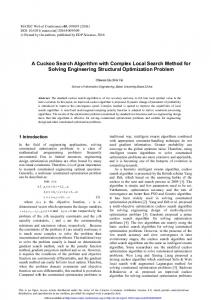
Figure 2: Expected Running Time (ERT, ) to reach fopt + ∆f and median number of function evaluations of successful trials (+), shown for ∆f = 10, 1, 10−1 , 10−2 , 10−3 , 10−5 , 10−8 (the exponent is given in the legend of f101 and f130 ) versus dimension in log-log presentation. The ERT(∆f ) equals to #FEs(∆f ) divided by the number of successful trials, where a trial is successful if fopt + ∆f was surpassed during the trial. The #FEs(∆f ) are the total number of function evaluations while fopt + ∆f was not surpassed during the trial from all respective trials (successful and unsuccessful), and fopt denotes the optimal function value. Crosses (×) indicate the total number of function evaluations #FEs(−∞). Numbers above ERT-symbols indicate the number of successful trials. Annotated numbers on the ordinate are decimal logarithms. Additional grid lines show linear and quadratic scaling.
•
2362
f 101 in 5-D,N=15,mFE=1977 f 101 in 20-D, N=15, mFE=10626 ∆f # ERT 10% 90% RTsucc # ERT 10% 90% RTsucc 10 15 7.6 e1 6.3 e1 9.0 e1 7.6 e1 15 1.0 e3 9.2 e2 1.1 e3 1.0 e3 1 15 2.8 e2 2.6 e2 2.9 e2 2.8 e2 15 2.2 e3 2.1 e3 2.4 e3 2.2 e3 1e−1 15 5.8 e2 5.6 e2 6.2 e2 5.8 e2 15 3.4 e3 3.3 e3 3.5 e3 3.4 e3 1e−3 15 9.4 e2 8.5 e2 1.0 e3 9.4 e2 15 5.5 e3 5.4 e3 5.6 e3 5.5 e3 1.4 e3 15 7.1 e3 7.0 e3 7.2 e3 7.1 e3 1e−5 15 1.4 e3 1.2 e3 1.5 e3 1e−8 15 1.8 e3 1.8 e3 1.8 e3 1.8 e3 15 9.3 e3 9.2 e3 9.5 e3 9.3 e3 f 103 in 5-D,N=15,mFE=5982 f 103 in 20-D, N=15, mFE=2000000 ∆f # ERT 10% 90% RTsucc # ERT 10% 90% RTsucc 10 15 6.6 e1 5.1 e1 8.1 e1 6.6 e1 15 9.3 e2 8.7 e2 9.9 e2 9.3 e2 1 15 3.1 e2 3.0 e2 3.3 e2 3.1 e2 15 2.1 e3 2.0 e3 2.2 e3 2.1 e3 1e−1 15 5.7 e2 5.4 e2 6.0 e2 5.7 e2 15 3.6 e3 3.5 e3 3.7 e3 3.6 e3 1e−3 15 1.0 e3 9.5 e2 1.1 e3 1.0 e3 15 7.9 e3 7.4 e3 8.3 e3 7.9 e3 1e−5 15 1.7 e3 1.6 e3 1.9 e3 1.7 e3 15 6.6 e4 4.4 e4 8.8 e4 6.6 e4 3.3 e3 2 1.4 e7 1.4 e7 1.5 e7 2.0 e6 1e−8 15 3.3 e3 2.9 e3 3.7 e3 f 105 in 5-D,N=15,mFE=125000 f 105 in 20-D, N=15, mFE=2000000 ∆f # ERT 10% 90% RTsucc # ERT 10% 90% RTsucc 10 15 6.4 e2 5.9 e2 6.9 e2 6.4 e2 1 2.8 e7 2.6 e7 3.0 e7 2.0 e6 12 8.4 e4 6.7 e4 1.0 e5 6.6 e4 1 3.0 e7 3.0 e7 3.0 e7 2.0 e6 1 1e−1 7 2.3 e5 2.1 e5 2.5 e5 1.1 e5 0 15e+0 12e+0 17e+0 1.3 e6 1e−3 5 3.3 e5 3.1 e5 3.6 e5 1.1 e5 . . . . . 1e−5 5 3.3 e5 3.1 e5 3.6 e5 1.1 e5 . . . . . 1.1 e5 . . . . . 1e−8 5 3.3 e5 3.1 e5 3.6 e5 f 107 in 5-D,N=15,mFE=12747 f 107 in 20-D, N=15, mFE=2000000 ∆f # ERT 10% 90% RTsucc # ERT 10% 90% RTsucc 10 15 7.6 e1 5.7 e1 9.6 e1 7.6 e1 15 9.2 e4 7.8 e4 1.1 e5 9.2 e4 1 15 1.1 e3 9.6 e2 1.3 e3 1.1 e3 15 3.6 e5 3.2 e5 4.0 e5 3.6 e5 3.1 e3 15 6.7 e5 6.2 e5 7.3 e5 6.7 e5 1e−1 15 3.1 e3 2.9 e3 3.3 e3 1e−3 15 6.5 e3 6.3 e3 6.8 e3 6.5 e3 15 1.2 e6 1.1 e6 1.3 e6 1.2 e6 1e−5 15 8.3 e3 7.9 e3 8.8 e3 8.3 e3 13 1.8 e6 1.7 e6 1.9 e6 1.5 e6 9.8 e3 1 3.0 e7 2.9 e7 3.0 e7 2.0 e6 1e−8 15 9.8 e3 9.2 e3 1.0 e4 f 109 in 5-D,N=15,mFE=125000 f 109 in 20-D, N=15, mFE=2000000 # ERT 10% 90% RTsucc # ERT 10% 90% RTsucc ∆f 10 15 6.3 e1 4.6 e1 8.0 e1 6.3 e1 15 1.3 e3 1.2 e3 1.4 e3 1.3 e3 15 3.3 e2 3.0 e2 3.6 e2 3.3 e2 15 3.1 e3 2.9 e3 3.3 e3 3.1 e3 1 1e−1 15 1.1 e3 1.0 e3 1.2 e3 1.1 e3 13 9.8 e5 7.3 e5 1.3 e6 8.0 e5 1e−3 15 1.2 e4 8.9 e3 1.4 e4 1.2 e4 0 54e–3 32e–3 10e–2 1.3 e6 1e−5 15 6.2 e4 5.1 e4 7.3 e4 6.2 e4 . . . . . 1.2 e5 . . . . . 1e−8 1 1.8 e6 1.8 e6 1.9 e6 f 111 in 5-D,N=15,mFE=125000 f 111 in 20-D, N=15, mFE=2000000 ∆f # ERT 10% 90% RTsucc # ERT 10% 90% RTsucc 10 15 9.6 e3 7.6 e3 1.2 e4 9.6 e3 0 17e+2 11e+2 24e+2 1.4 e6 1 2 8.6 e5 7.8 e5 9.4 e5 7.4 e4 . . . . . 7.1 e4 . . . . . 1e−1 0 19e–1 98e–2 33e–1 1e−3 . . . . . . . . . . . . . . . . . . . 1e−5 . 1e−8 . . . . . . . . . . f 113 in 5-D,N=15,mFE=125000 f 113 in 20-D, N=15, mFE=2000000 ∆f # ERT 10% 90% RTsucc # ERT 10% 90% RTsucc 10 15 2.9 e2 2.1 e2 3.8 e2 2.9 e2 11 1.3 e6 9.6 e5 1.7 e6 1.0 e6 1 15 2.9 e3 2.5 e3 3.3 e3 2.9 e3 0 62e–1 29e–1 17e+0 1.1 e6 1e−1 13 4.0 e4 2.2 e4 5.9 e4 3.0 e4 . . . . . 1e−3 8 1.3 e5 9.7 e4 1.7 e5 7.0 e4 . . . . . 1e−5 8 1.3 e5 9.7 e4 1.6 e5 7.0 e4 . . . . . 1e−8 8 1.3 e5 1.0 e5 1.7 e5 7.0 e4 . . . . . f 115 in 5-D,N=15,mFE=125000 f 115 in 20-D, N=15, mFE=2000000 # ERT 10% 90% RTsucc # ERT 10% 90% RTsucc ∆f 10 15 1.9 e2 1.6 e2 2.2 e2 1.9 e2 15 1.4 e4 6.4 e3 2.1 e4 1.4 e4 1 15 1.6 e3 1.1 e3 2.1 e3 1.6 e3 2 1.4 e7 1.3 e7 1.5 e7 1.6 e6 1e−1 12 5.5 e4 3.5 e4 7.7 e4 3.2 e4 0 15e–1 99e–2 33e–1 1.0 e6 1.2 e5 . . . . . 1e−3 4 3.9 e5 3.4 e5 4.4 e5 1e−5 4 3.9 e5 3.3 e5 4.4 e5 1.2 e5 . . . . . 1.2 e5 . . . . . 1e−8 1 1.8 e6 1.6 e6 1.9 e6 f 117 in 5-D,N=15,mFE=125000 f 117 in 20-D, N=15, mFE=2000000 # ERT 10% 90% RTsucc # ERT 10% 90% RTsucc ∆f 10 13 5.8 e4 4.4 e4 7.2 e4 5.3 e4 0 36e+2 26e+2 59e+2 8.9 e5 1 1 1.8 e6 1.7 e6 1.9 e6 1.2 e5 . . . . . 1e−1 0 27e–1 12e–1 12e+0 8.9 e4 . . . . . 1e−3 . . . . . . . . . . 1e−5 . . . . . . . . . . 1e−8 . . . . . . . . . . f 119 in 5-D,N=15,mFE=125000 f 119 in 20-D, N=15, mFE=2000000 ∆f # ERT 10% 90% RTsucc # ERT 10% 90% RTsucc 10 15 1.9 e1 1.5 e1 2.3 e1 1.9 e1 15 7.0 e3 5.7 e3 8.5 e3 7.0 e3 1 15 8.3 e2 6.3 e2 1.0 e3 8.3 e2 10 1.4 e6 9.9 e5 1.8 e6 8.6 e5 1e−1 15 4.5 e3 4.0 e3 5.0 e3 4.5 e3 4 6.8 e6 6.3 e6 7.3 e6 1.8 e6 1e−3 15 1.3 e4 1.2 e4 1.5 e4 1.3 e4 0 13e–2 60e–3 33e–1 1.6 e6 1e−5 8 1.6 e5 1.4 e5 1.9 e5 1.0 e5 . . . . . 1e−8 0 61e–7 12e–7 42e–6 7.1 e4 . . . . .
f 102 in 5-D,N=15,mFE=1954 f 102 in 20-D, N=15, mFE=11485 # ERT 10% 90% RTsucc # ERT 10% 90% RTsucc 15 7.7 e1 6.2 e1 9.0 e1 7.7 e1 15 1.2 e3 1.1 e3 1.2 e3 1.2 e3 15 2.9 e2 2.6 e2 3.2 e2 2.9 e2 15 2.5 e3 2.4 e3 2.7 e3 2.5 e3 15 5.8 e2 5.1 e2 6.4 e2 5.8 e2 15 4.0 e3 3.9 e3 4.2 e3 4.0 e3 15 9.7 e2 8.6 e2 1.1 e3 9.7 e2 15 5.9 e3 5.8 e3 6.1 e3 5.9 e3 15 1.3 e3 1.2 e3 1.5 e3 1.3 e3 15 7.6 e3 7.4 e3 7.8 e3 7.6 e3 15 1.8 e3 1.8 e3 1.8 e3 1.8 e3 15 9.8 e3 9.5 e3 1.0 e4 9.8 e3 f 104 in 5-D,N=15,mFE=17794 f 104 in 20-D, N=15, mFE=2000000 ∆f # ERT 10% 90% RTsucc # ERT 10% 90% RTsucc 10 15 6.3 e2 6.0 e2 6.6 e2 6.3 e2 2 1.4 e7 1.3 e7 1.5 e7 1.3 e6 1 15 5.5 e3 4.2 e3 6.8 e3 5.5 e3 0 14e+0 82e–1 15e+0 1.8 e6 1e−1 15 6.6 e3 5.3 e3 8.0 e3 6.6 e3 . . . . . 1e−3 15 7.8 e3 6.6 e3 9.0 e3 7.8 e3 . . . . . 1e−5 15 8.4 e3 7.2 e3 9.8 e3 8.4 e3 . . . . . 8.9 e3 . . . . . 1e−8 15 8.9 e3 7.7 e3 1.0 e4 f 106 in 5-D,N=15,mFE=35488 f 106 in 20-D, N=15, mFE=2000000 ∆f # ERT 10% 90% RTsucc # ERT 10% 90% RTsucc 10 15 5.8 e2 5.7 e2 5.9 e2 5.8 e2 15 9.4 e4 8.1 e4 1.1 e5 9.4 e4 15 2.1 e3 1.8 e3 2.3 e3 2.1 e3 15 3.9 e5 3.2 e5 4.6 e5 3.9 e5 1 1e−1 15 3.9 e3 3.3 e3 4.6 e3 3.9 e3 15 6.8 e5 5.8 e5 7.9 e5 6.8 e5 1e−3 15 7.4 e3 6.3 e3 8.7 e3 7.4 e3 1 2.9 e7 2.8 e7 3.0 e7 2.0 e6 1e−5 15 1.0 e4 8.3 e3 1.2 e4 1.0 e4 0 15e–3 11e–4 59e–3 7.9 e5 1.6 e4 . . . . . 1e−8 15 1.6 e4 1.3 e4 1.8 e4 f 108 in 5-D,N=15,mFE=125000 f 108 in 20-D, N=15, mFE=2000000 ∆f # ERT 10% 90% RTsucc # ERT 10% 90% RTsucc 10 15 1.1 e2 8.6 e1 1.4 e2 1.1 e2 0 21e+0 15e+0 26e+0 1.0 e6 1 15 5.2 e3 3.6 e3 6.8 e3 5.2 e3 . . . . . 5.2 e4 . . . . . 1e−1 14 5.6 e4 4.4 e4 6.8 e4 1e−3 0 29e–3 44e–4 81e–3 1.0 e5 . . . . . 1e−5 . . . . . . . . . . . . . . . . . . . 1e−8 . f 110 in 5-D,N=15,mFE=125000 f 110 in 20-D, N=15, mFE=2000000 # ERT 10% 90% RTsucc # ERT 10% 90% RTsucc ∆f 10 15 1.8 e3 1.6 e3 2.0 e3 1.8 e3 0 28e+0 24e+0 31e+0 1.6 e6 4 3.5 e5 3.0 e5 4.1 e5 9.6 e4 . . . . . 1 1e−1 1 1.8 e6 1.8 e6 1.9 e6 1.2 e5 . . . . . 1e−3 0 15e–1 11e–2 21e–1 5.6 e4 . . . . . 1e−5 . . . . . . . . . . . . . . . . . . . 1e−8 . f 112 in 5-D,N=15,mFE=125000 f 112 in 20-D, N=15, mFE=2000000 ∆f # ERT 10% 90% RTsucc # ERT 10% 90% RTsucc 10 15 5.8 e2 5.6 e2 6.0 e2 5.8 e2 0 16e+0 12e+0 17e+0 7.9 e5 1 15 2.6 e4 1.3 e4 3.8 e4 2.6 e4 . . . . . 1.0 e5 . . . . . 1e−1 4 3.9 e5 3.4 e5 4.4 e5 1e−3 1 1.8 e6 1.6 e6 1.9 e6 1.2 e5 . . . . . 8.9 e4 . . . . . 1e−5 0 28e–2 13e–3 68e–2 1e−8 . . . . . . . . . . f 114 in 5-D,N=15,mFE=125000 f 114 in 20-D, N=15, mFE=2000000 ∆f # ERT 10% 90% RTsucc # ERT 10% 90% RTsucc 10 15 9.7 e2 6.0 e2 1.4 e3 9.7 e2 0 67e+0 57e+0 79e+0 1.0 e6 1 15 2.3 e4 1.6 e4 3.0 e4 2.3 e4 . . . . . 1e−1 5 3.3 e5 3.1 e5 3.5 e5 1.1 e5 . . . . . 1e−3 0 29e–2 47e–3 69e–2 7.9 e4 . . . . . 1e−5 . . . . . . . . . . 1e−8 . . . . . . . . . . f 116 in 5-D,N=15,mFE=125000 f 116 in 20-D, N=15, mFE=2000000 # ERT 10% 90% RTsucc # ERT 10% 90% RTsucc ∆f 10 14 1.5 e4 5.7 e3 2.5 e4 1.4 e4 0 57e+1 39e+1 11e+2 1.6 e6 1 10 8.0 e4 5.6 e4 1.1 e5 5.1 e4 . . . . . 1e−1 5 3.1 e5 2.6 e5 3.4 e5 1.2 e5 . . . . . 7.1 e4 . . . . . 1e−3 0 37e–2 14e–3 38e–1 1e−5 . . . . . . . . . . . . . . . . . . . 1e−8 . f 118 in 5-D,N=15,mFE=125000 f 118 in 20-D, N=15, mFE=2000000 # ERT 10% 90% RTsucc # ERT 10% 90% RTsucc ∆f 10 15 1.8 e3 1.5 e3 2.1 e3 1.8 e3 7 3.3 e6 2.9 e6 3.7 e6 1.2 e6 1 15 1.7 e4 6.0 e3 2.9 e4 1.7 e4 0 10e+0 42e–1 29e+0 1.0 e6 1e−1 13 6.8 e4 5.1 e4 8.7 e4 5.5 e4 . . . . . 1e−3 6 2.6 e5 2.3 e5 2.9 e5 9.8 e4 . . . . . 1e−5 2 8.9 e5 8.4 e5 9.4 e5 1.2 e5 . . . . . 1e−8 0 33e–4 43e–7 16e–2 8.9 e4 . . . . . f 120 in 5-D,N=15,mFE=125000 f 120 in 20-D, N=15, mFE=2000000 ∆f # ERT 10% 90% RTsucc # ERT 10% 90% RTsucc 10 15 1.7 e1 1.1 e1 2.1 e1 1.7 e1 15 4.6 e4 3.0 e4 6.5 e4 4.6 e4 1 15 3.4 e3 1.8 e3 5.1 e3 3.4 e3 0 56e–1 41e–1 77e–1 1.0 e6 1e−1 11 9.6 e4 7.6 e4 1.1 e5 6.4 e4 . . . . . 1e−3 0 34e–3 89e–4 40e–2 7.9 e4 . . . . . 1e−5 . . . . . . . . . . 1e−8 . . . . . . . . . . ∆f 10 1 1e−1 1e−3 1e−5 1e−8
Table 1: Shown are, for functions f101 -f120 and for a given target difference to the optimal function value ∆f : the number of successful trials (#); the expected running time to surpass fopt + ∆f (ERT, see Figure 2); the 10%-tile and 90%-tile of the bootstrap distribution of ERT; the average number of function evaluations in successful trials or, if none was successful, as last entry the median number of function evaluations to reach the best function value (RTsucc ). If fopt + ∆f was never reached, figures in italics denote the best achieved ∆f -value of the median trial and the 10% and 90%-tile trial. Furthermore, N denotes the number of trials, and mFE denotes the maximum of number of function evaluations executed in one trial. See Figure 2 for the names of functions.
2363
D=5 1.0 +1:30/30
D = 20 1.0
f101-130
f101-130
0.8
-8:12/30 0.6
0.4
0.2
0.0 0
1
2
+1:6/6
-8:4/30 0.6
0.4
3
4
0
1
2
3
4
5
6
7
8
9
0.0 0
10 11 12 13 14
f101-130 1
log10 of Df / Dftarget
2
3
4
1.0
f101-106
proportion of trials
0.4
0.2
1
2
1.0 +1:15/15
3
4
0
1
2
3
0.8
4
5
6
7
8
9
10 11 12 13 14
-4:3/6 -8:3/6
0.6
0.4
4
5
6
7
8
9
0.0 0
10 11 12 13 14
f101-106 1
log10 of Df / Dftarget
2
3
4
5
0
1
2
3
log10 of FEvals / DIM
1.0
f107-121
4
5
6
7
8
9
10 11 12 13 14
log10 of Df / Dftarget
f107-121
+1:8/15 -1:4/15
-4:6/15
proportion of trials
proportion of trials
3
log10 of Df / Dftarget
-1:13/15
severe noise
2
0.2
f101-106 log10 of FEvals / DIM
-8:4/15
0.6
0.4
0.2
-4:1/15
0.8
-8:1/15
0.6
0.4
0.2
f107-121 1
2
3
4
0
1
2
3
log10 of FEvals / DIM
1.0
4
5
6
7
8
9
0.0 0
10 11 12 13 14
f107-121 1
log10 of Df / Dftarget
2
3
4
5
0
1
2
3
log10 of FEvals / DIM
1.0
f122-130
4
5
6
7
8
9
10 11 12 13 14
log10 of Df / Dftarget
f122-130
+1:8/9 -1:1/9
0.8
proportion of trials
proportion of trials
severe noise multimod.
1
-1:4/6
-8:6/6
0.0 0
0
f101-106
+1:6/6
-4:6/6
0.6
0.8
5
log10 of FEvals / DIM
-1:6/6
proportion of trials
moderate noise
1.0
0.0 0
-4:4/30
0.8
0.2
f101-130 log10 of FEvals / DIM
0.8
+1:22/30 -1:9/30
-4:15/30
proportion of trials
proportion of trials
all functions
-1:27/30
0.6
0.4 +1:9/9 0.2
-1:8/9
0.8
-4:0/9 -8:0/9
0.6
0.4
0.2
-4:3/9 -8:2/9 0.0 0
1
f122-130 2
3
log10 of FEvals / DIM
4
0
1
2
3
4
5
6
7
8
9
0.0 0
10 11 12 13 14
log10 of Df / Dftarget
f122-130 1
2
3
log10 of FEvals / DIM
4
5
0
1
2
3
4
5
6
7
8
9
10 11 12 13 14
log10 of Df / Dftarget
Figure 3: Empirical cumulative distribution functions (ECDFs), plotting the fraction of trials versus running time (left) or ∆f . Left subplots: ECDF of the running time (number of function evaluations), divided by search space dimension D, to fall below fopt + ∆f with ∆f = 10k , where k is the first value in the legend. Right subplots: ECDF of the best achieved ∆f divided by 10k (upper left lines in continuation of the left subplot), and best achieved ∆f divided by 10−8 for running times of D, 10 D, 100 D . . . function evaluations (from right to left cycling black-cyan-magenta). Top row: all results from all functions; second row: moderate noise functions; third row: severe noise functions; fourth row: severe noise and highly-multimodal functions. The legends indicate the number of functions that were solved in at least one trial. FEvals denotes number of function evaluations, D and DIM denote search space dimension, and ∆f and Df denote the difference to the optimal function value.
2364
∆f 10 1 1e−1 1e−3 1e−5 1e−8 ∆f 10 1 1e−1 1e−3 1e−5 1e−8 ∆f 10 1 1e−1 1e−3 1e−5 1e−8 ∆f 10 1 1e−1 1e−3 1e−5 1e−8 ∆f 10 1 1e−1 1e−3 1e−5 1e−8
f 121 in 5-D,N=15,mFE=125000 # ERT 10% 90% RTsucc 15 2.4 e1 2.0 e1 2.9 e1 2.4 e1 15 4.1 e2 3.3 e2 5.0 e2 4.1 e2 15 1.4 e3 1.2 e3 1.7 e3 1.4 e3 8 1.9 e5 1.7 e5 2.1 e5 1.0 e5 0 99e–5 18e–5 29e–4 8.9 e4 . . . . . f 123 in 5-D,N=15,mFE=125000 # ERT 10% 90% RTsucc 15 1.5 e1 1.2 e1 1.8 e1 1.5 e1 14 3.9 e4 2.6 e4 5.3 e4 3.8 e4 0 64e–2 52e–2 97e–2 3.5 e4 . . . . . . . . . . . . . . . f 125 in 5-D,N=15,mFE=125000 # ERT 10% 90% RTsucc 15 1.3 e0 1.1 e0 1.5 e0 1.3 e0 15 3.5 e1 2.6 e1 4.5 e1 3.5 e1 15 4.7 e3 3.3 e3 6.5 e3 4.7 e3 0 80e–4 33e–4 19e–3 8.9 e4 . . . . . . . . . . f 127 in 5-D,N=15,mFE=125000 # ERT 10% 90% RTsucc 15 1.2 e0 1.1 e0 1.3 e0 1.2 e0 15 3.9 e1 3.0 e1 4.8 e1 3.9 e1 15 8.6 e3 5.6 e3 1.2 e4 8.6 e3 0 32e–3 86e–4 51e–3 6.3 e4 . . . . . . . . . . f 129 in 5-D,N=15,mFE=125000 # ERT 10% 90% RTsucc 15 9.8 e1 7.2 e1 1.2 e2 9.8 e1 15 1.1 e4 6.0 e3 1.6 e4 1.1 e4 11 9.3 e4 7.2 e4 1.1 e5 7.9 e4 1 1.8 e6 1.8 e6 1.9 e6 1.2 e5 1 1.8 e6 1.8 e6 1.9 e6 1.2 e5 0 16e–3 10e–4 26e–2 6.3 e4
f 121 in 20-D, N=15, mFE=2000000 # ERT 10% 90% RTsucc 15 9.7 e2 8.9 e2 1.1 e3 9.7 e2 15 7.4 e4 4.1 e4 1.1 e5 7.4 e4 2 1.4 e7 1.3 e7 1.5 e7 2.0 e6 0 18e–2 88e–3 25e–2 8.9 e5 . . . . . . . . . . f 123 in 20-D, N=15, mFE=2000000 # ERT 10% 90% RTsucc 15 1.1 e3 7.1 e2 1.5 e3 1.1 e3 0 45e–1 36e–1 55e–1 1.3 e6 . . . . . . . . . . . . . . . . . . . . f 125 in 20-D, N=15, mFE=2000000 # ERT 10% 90% RTsucc 15 1.2 e0 1.1 e0 1.3 e0 1.2 e0 15 1.5 e3 1.3 e3 1.7 e3 1.5 e3 0 39e–2 36e–2 42e–2 1.0 e6 . . . . . . . . . . . . . . . f 127 in 20-D, N=15, mFE=2000000 # ERT 10% 90% RTsucc 15 1.1 e0 1.0 e0 1.1 e0 1.1 e0 15 4.2 e2 3.3 e2 5.1 e2 4.2 e2 0 43e–2 34e–2 49e–2 1.3 e6 . . . . . . . . . . . . . . . f 129 in 20-D, N=15, mFE=2000000 # ERT 10% 90% RTsucc 0 27e+0 24e+0 42e+0 1.3 e6 . . . . . . . . . . . . . . . . . . . . . . . . .
∆f 10 1 1e−1 1e−3 1e−5 1e−8 ∆f 10 1 1e−1 1e−3 1e−5 1e−8 ∆f 10 1 1e−1 1e−3 1e−5 1e−8 ∆f 10 1 1e−1 1e−3 1e−5 1e−8 ∆f 10 1 1e−1 1e−3 1e−5 1e−8
f 122 in 5-D,N=15,mFE=125000 # ERT 10% 90% RTsucc 15 1.6 e1 8.9 e0 2.4 e1 1.6 e1 15 7.5 e3 4.9 e3 1.0 e4 7.5 e3 15 4.5 e4 4.0 e4 5.0 e4 4.5 e4 1 1.8 e6 1.8 e6 1.9 e6 1.2 e5 0 76e–4 15e–4 46e–3 1.1 e5 . . . . . f 124 in 5-D,N=15,mFE=125000 # ERT 10% 90% RTsucc 15 1.7 e1 1.1 e1 2.5 e1 1.7 e1 15 1.0 e3 8.5 e2 1.2 e3 1.0 e3 2 9.0 e5 8.7 e5 9.4 e5 1.2 e5 0 20e–2 87e–3 37e–2 8.9 e4 . . . . . . . . . . f 126 in 5-D,N=15,mFE=125000 # ERT 10% 90% RTsucc 15 1.1 e0 1.0 e0 1.1 e0 1.1 e0 15 3.5 e1 2.6 e1 4.5 e1 3.5 e1 15 9.4 e3 7.6 e3 1.1 e4 9.4 e3 0 27e–3 89e–4 45e–3 7.1 e4 . . . . . . . . . . f 128 in 5-D,N=15,mFE=51751 # ERT 10% 90% RTsucc 15 1.2 e2 9.6 e1 1.5 e2 1.2 e2 15 5.5 e3 4.2 e3 6.9 e3 5.5 e3 15 9.9 e3 7.7 e3 1.2 e4 9.9 e3 15 1.9 e4 1.5 e4 2.4 e4 1.9 e4 15 2.4 e4 1.9 e4 2.8 e4 2.4 e4 15 2.9 e4 2.4 e4 3.3 e4 2.9 e4 f 130 in 5-D,N=15,mFE=125000 # ERT 10% 90% RTsucc 15 1.3 e2 1.0 e2 1.7 e2 1.3 e2 14 2.2 e4 9.2 e3 3.6 e4 2.2 e4 11 5.2 e4 3.0 e4 7.4 e4 4.9 e4 11 7.0 e4 4.5 e4 9.6 e4 5.7 e4 11 8.4 e4 6.2 e4 1.1 e5 6.7 e4 8 1.6 e5 1.3 e5 1.8 e5 1.0 e5
f 122 in 20-D, N=15, mFE=2000000 # ERT 10% 90% RTsucc 15 7.1 e2 4.2 e2 1.0 e3 7.1 e2 0 27e–1 17e–1 36e–1 1.1 e6 . . . . . . . . . . . . . . . . . . . . f 124 in 20-D, N=15, mFE=2000000 # ERT 10% 90% RTsucc 15 2.3 e2 2.0 e2 2.6 e2 2.3 e2 1 3.0 e7 3.0 e7 3.0 e7 2.0 e6 0 16e–1 12e–1 19e–1 1.3 e6 . . . . . . . . . . . . . . . f 126 in 20-D, N=15, mFE=2000000 # ERT 10% 90% RTsucc 15 1.1 e0 1.0 e0 1.1 e0 1.1 e0 15 2.5 e3 2.1 e3 2.9 e3 2.5 e3 0 52e–2 38e–2 54e–2 1.0 e6 . . . . . . . . . . . . . . . f 128 in 20-D, N=15, mFE=2000000 # ERT 10% 90% RTsucc 1 3.0 e7 3.0 e7 3.0 e7 2.0 e6 0 30e+0 22e+0 36e+0 1.4 e6 . . . . . . . . . . . . . . . . . . . . f 130 in 20-D, N=15, mFE=2000000 # ERT 10% 90% RTsucc 15 1.2 e5 5.5 e4 2.0 e5 1.2 e5 3 8.1 e6 6.8 e6 9.4 e6 1.3 e6 3 8.2 e6 6.9 e6 9.4 e6 1.4 e6 1 3.0 e7 3.0 e7 3.0 e7 2.0 e6 0 21e–1 40e–4 49e–1 1.4 e6 . . . . .
Table 2: Shown are, for functions f121 -f130 and for a given target difference to the optimal function value ∆f : the number of successful trials (#); the expected running time to surpass fopt + ∆f (ERT, see Figure 2); the 10%-tile and 90%-tile of the bootstrap distribution of ERT; the average number of function evaluations in successful trials or, if none was successful, as last entry the median number of function evaluations to reach the best function value (RTsucc ). If fopt + ∆f was never reached, figures in italics denote the best achieved ∆f -value of the median trial and the 10% and 90%-tile trial. Furthermore, N denotes the number of trials, and mFE denotes the maximum of number of function evaluations executed in one trial. See Figure 2 for the names of functions.
[10]
[11]
[12]
[13]
[14]
[15]
X. Y. at al., editor, Parallel Problem Solving for Nature - PPSN VIII, LNCS 3242, pages 282–291. Springer, 2004. N. Hansen, S. M¨ uller, and P. Koumoutsakos. Reducing the Time Complexity of the Derandomized Evolution Strategy with Covariance Matrix Adaptation (CMA-ES). Evolutionary Computation, 1(11):1–18, 2003. N. Hansen and A. Ostermeier. Adapting Arbitrary Normal Mutation Distributions in Evolution Strategies: The Covariance Matrix Adaptation. In Proceeding of the IEEE International Conference on Evolutionary Computation (ICEC ’96), pages 312–317, 1996. W. Hart. Adaptive Global Optimization With Local Search. PhD thesis, Univ. California, San Diego, CA., 1994. N. Krasnogor and J. Smith. A Tutorial for Competent Memetic Algorithms: Model, Taxonomy, and Design Issue. IEEE Transactions on Evolutionary Computation, 9(5):474–488, 2005. M. S. Land. Evolutionary Algorithms with Local Search for Combinational Optimization. PhD thesis, Univ. California, San Diego, CA., 1998. P. Merz. Memetic Algorithms for Combinational Optimization Problems: Fitness Landscapes and Effective Search Strategies. PhD thesis, Gesamthochschule Siegen, University of Siegen, Germany, 2000.
[16] D. Molina, M. Lozano, C. Garc´ıa-Mart´ınez, and F. Herrera. Memetic algorithms for continuous optimization based on local search chains. Evolutionary Computation. In press, 2009. [17] P. Moscato. On evolution, search, optimization, genetic algorithms and martial arts: Towards memetic algorithms. Technical report, Technical Report Caltech Concurrent Computation Program Report 826, Caltech, Pasadena, California, 1989. [18] P. Moscato. Memetic algorithms: a short introduction, pages 219–234. McGraw-Hill, London, 1999. [19] P. Suganthan, N. Hansen, J. Liang, K. Deb, Y. Chen, A. Auger, and S. Tiwari. Problem definitions and evaluation criteria for the CEC 2005 special session on real parameter optimization. Technical report, Nanyang Technical University, 2005. [20] G. Syswerda. Uniform Crossover in Genetic Algorithms. In J. D. Schaffer, editor, Proc. of the Thrid Int. Conf. on Genetic Algorithms, pages 2–9. Morgan Kaufmann Publishers, San Mateo, 1989. [21] E. Talbi. A Taxonomy of Hybrid Metaheuristics. Journal of Heuristics, 8:541–564, 2002.
2365