Progress In Electromagnetics Research B, Vol. 33, 115–134, 2011
A METHOD FOR TRACKING CHARACTERISTIC NUMBERS AND VECTORS M. Capek* , P. Hazdra, P. Hamouz, and J. Eichler Department of Electromagnetic Field, Faculty of Electrical Engineering, Czech Technical University in Prague, Technicka 2, 16627 Prague 6, Czech Republic Abstract—A new method for tracking characteristic numbers and vectors appearing in the Characteristic Mode Theory is presented in this paper. The challenge here is that the spectral decomposition of the moment impedance-matrix doesn’t always produce well ordered eigenmodes. This issue is addressed particularly to finite numerical accuracy and slight nonsymmetry of the frequencydependent matrix. At specific frequencies, the decomposition problem might be ill-posed and non-uniquely defined as well. Hence an advanced tracking procedure has been developed to deal with noisy modes, non-continuous behavior of eigenvalues, mode swapping etc. Proposed method has been successfully implemented into our in-house Characteristic Mode software tool for the design of microstrip patch antennas and tested for some interesting examples. 1. INTRODUCTION Eigenmodes and eigenvalues are valuable characteristics of important electromagnetic operators like Electric Field Integral Equation EFIE [1]. After necessary numerical processing (as the analytical solution is available for only few canonical cases, [2]), those functional operators become discrete and are conventionally represented by a matrix [3]. Diagonalization techniques like the spectral matrix decomposition [4] or the Singular Value Decomposition (SVD) [5] are capable to obtain an orthogonal set of eigenmodes which are of great physical importance [6]. In the following text, spectral eigendecomposition of the EFIE complex impedance matrix is performed in the frequency domain over a relatively broadband sweep (through several resonances). Received 2 June 2011, Accepted 18 July 2011, Scheduled 28 July 2011 * Corresponding author: Miloslav Capek (
[email protected]).
116
Capek et al.
Unfortunately, it is found that modes and eigenvalues are not generally sorted properly with frequency. Mode order might be switched, or an unphysical solution arises. Moreover, some modes could turn up (or disappear) at any frequency step. We recognize the proper manipulation and tracking of the modes as the main problem when dealing with modal decomposition, namely the Theory of Characteristic Modes (TCM) [7]. Straightforward method used so far, based on simple eigenvector correlation, has been found insufficient for complex structures. 2. MATHEMATICAL FORMULATION OF THEORY OF CHARACTERISTIC MODES The tangential electric field on a Perfect Electrical Conductor (PEC) satisfies the equation Estan + Eitan = 0, (1) where index s represents the scattered field and index i the incident field respectively. Since the radiated field Estan is a function of the induced surface current density J, the following integral operator L is introduced: L(J) = Estan . (2) Combining 1 and 2 we arrive at the so-called EFIE (Electric Field Integral Equation) [8]: £ ¤ L(J) − Ei tan = 0. (3) The potential structure of the L(J) operator is well-known and may be found e.g., in [9]. Since L relates field and current quantities, it has a character of impedance: Z(J) = [L(J)]tan
(4)
and in discrete form the above is known as the Method of Moments complex impedance matrix Z = R + jX. For TCM modaldecomposition purposes, this matrix has to be symmetrical with its real and imaginary Hermitian parts [10]. Thus, the Galerkin method [11] is required for the construction of Z. Let us consider the following functional relation: F (J) =
hJ, XJi power stored = . hJ, RJi power radiated
(5)
There exists a set of modal currents (called the characteristic ones) that minimize the above functional. These characteristic currents are thus maximizing the power radiated by the structure. It is known
Progress In Electromagnetics Research B, Vol. 33, 2011
117
that (5) could be minimized by solving the associated Euler’s equation (weighted eigen-equation): XJn = λn RJn ,
(6)
where Jn are real characteristic currents and λn their associated eigenvalues [12]. Instead of eigenvalues, characteristic angles are being used often thanks to their steeper change: αn = 180 − arctan(λn ).
(7)
Characteristic angles are (theoretically) continuous through the values of 90–270, resonance of the nth mode occurs when αn = 180. An illustration example of λn and αn for a simple strip dipole antenna is shown at Fig. 1, the pink horizontal line marks the resonance. Halfwave dipole has been simulated as 300 mm long strip dipole of 5 mm width.
f [GHz]
Figure 1. Eigenvalues and characteristic angles for simple strip dipole 300 × 5 mm, 6 modes. The TCM has been implemented into Matlab’s code. The EFIE core is based on the RWG elements [13]. 3. THE TRACKING PROBLEM By the numerical solution of (6) in Matlab (particularly by the eig function that make use of the LAPACK [14] package), eigenvalues and eigenvectors are obtained. The sorting problem is schematically depicted at Fig. 2 — during sequential frequency steps, mode order swaps (red arrows) or modes arise or vanish. This quite typical behavior is illustrated on an example of rectangular perfectly
118
Capek et al.
(a)
(b)
Figure 2. The tracking problem. Original data from TCM (a) and ideally sorted results (b).
Figure 3. Unsorted characteristic currents for rectangular plate (modes 1. and 2. are swapping at 2nd and 3rd sample, mode 3 at 3rd position is corrupted). conductive plate — see a few unsorted modes at Fig. 3. Clearly, the eigenvalues are swapped, so there are physically different current distributions along the frequency. Let’s demonstrate our effort on three examples of different structural and computational complexity. First is a 100 × 60 mm rectangle (further noted as Rec100 × 60, Fig. 4(a)), discretized with 244 triangular RWG elements. Eigenvalues have been calculated for frequencies 1 GHz–4 GHz with 50 MHz steps. For this simple case there are no serious sorting problems. The second example is represented by 110 × 30 mm U-slot patch antenna [15] (Fig. 4(b)) with 722 triangles and 161 frequency steps between 0.5 GHz and 4.5 GHz. The last (and
Progress In Electromagnetics Research B, Vol. 33, 2011
(a)
(b)
119
(c)
Figure 4. Demonstration examples (rectangle plate, U slot patch antenna and fractal antenna). probably most interesting) example that will be discussed is the fractal patch antenna of 2nd iteration. Fractal motif is based on the “X” motif [16] (further noted as FRC B2, Fig. 4(c)). The FRC B2 fractal is discretized into 518 elements and computed at frequencies 0.7 GHz– 2.8 GHz with 20 MHz steps. For the U-slot antenna and fractal patch antenna, infinite ground plane was considered (height of patches above the ground plane is 12 mm and 10 mm, respectively). It will be shown that initial simple eigenvector correlation approach (described later in Section 3.2) fails for such complex structures as this fractal one. 3.1. The Tracking Problem Definition As already shown at Fig. 2 and Fig. 3, eigenvalues and eigenvectors are more or less randomly swapped and they need to be properly sorted. There are also other, accuracy-related, problems: matrix numerical noise (rounding errors) and matrix symmetry. 3.1.1. Eigenvalues These numerical issues lead to ±∞ or 0 valued eigenvalues at certain frequencies. But fortunately, the frequency behaviour of eigenvalues could be interpolated later. Occasionally, some eigenvalues suddenly changes their sign (see later). Although the MoM code is based on the Galerkin testing procedure, the Z-matrix is not purely symmetrical [17]. As a result, some eigenvalues have unphysical imaginary parts which should be cut off. Another complication originates from the fact that the user may request more modes than are available at a given frequency. Such empty positions are replaced by the “NaN” values for further manipulation and user notification.
120
Capek et al.
3.1.2. Eigenvectors
α[ ]
α[ ]
Problems with eigenvectors are weaker because they are directly used as the input data for tracking. Three main complications were recognized in eigenvectors context: zero vectors, numerical noise (chaotic modes) and degenerated modes. All the above described numerical problems significantly complicate the respective tracking. Fig. 5 and Fig. 6 shows raw unsorted characteristic angles for Rec100 × 60, U-slot antenna and FRC B2. It could be seen that there are frequent leaps as sketched at Fig. 2. Abrupt jumps to values of 90 or 270 are due to the +/− sign changes of characteristic numbers.
ο
ο
f [GHz]
f [GHz]
(a)
(b)
α[ ]
α[ ]
Figure 5. Unsorted raw characteristic angles ((a) Rec100 × 60, (b) Uslot).
ο
ο
f [GHz]
(a)
f [GHz]
(b)
Figure 6. Unsorted raw characteristic angles ((a) FRC B2 and (b) the detail at 2.1 GHz–2.8 GHz), only the first three modes are shown for clarity.
Progress In Electromagnetics Research B, Vol. 33, 2011
121
3.2. Previous Tracking Method Previous tracking method was based on the correlation of the characteristic vectors (corrcoef in Matlab). Modes are sorted in eigenvalue-ascending order from the lowest frequency. Initially, modes from the first frequency are simply copied from the unsorted array to the sorted one. For all the combinations of modes on the first frequency and subsequent (yet unsorted) frequencies, the correlation coefficients of eigenvectors are calculated. For each mode on the first frequency, we find its next frequency pair with the highest respective correlation coefficient. Modes are then copied into an array dedicated for sorted modes and this procedure is repeated for all the frequencies in ascending order (see Fig. 7). The above method is very simple because there is no need for any preprocessing — we work with eigenvectors directly obtained from the
α[ ]
α[ ]
Figure 7. The schematic procedure for sorting using the correlation method and assigning the mode with the min. correlation coefficient (modes are represented by the char. number).
ο
ο
f [GHz]
(a)
f [GHz]
(b)
Figure 8. (a) The sorted characteristic angles (correlation method) for Rec100 × 60 and (b) U-slot antenna.
Capek et al.
α[ ]
α[ ]
122
ο
ο
f [GHz]
(b) f [GHz]
f [GHz]
(a)
(b)
Figure 9. (a) The sorted characteristic angles (correlation method) for FRC B2 and (b) the detail at 2.1 GHz–2.8 GHz, same structure. Compare these results with the unsorted data at Fig. 6 to notice swapping and missing modes. eig function. All modes are treated as existing from the 1st frequency sample to the end of the tracking process. For simple structures, this approach is quite satisfactory (see Fig. 8 for rectangle without and with U-slot). For advanced structures, however, modes can easily “swap”, or one mode might merge with another one; thereupon the mode goes missing on the remaining frequencies (Fig. 9, FRC B2 (b)). 3.3. New Method The new proposed tracking method is split into three stages — preprocessing of raw data from the eig function, main sorting and postprocessing (mode discrimination, eigenvalue interpolation and refining). Contrary to the correlation method described in Section 3.2, more tricks have had been employed, one of the basic precautions is that the Z-matrix is now calculated in double-precision. A slight increase in solving time (5–10%) is compensated by much precise sorting. Since the new tracking method algorithm is rather extensive, please follow the flowchart of the whole procedure shown at Fig. 10. 3.4. New Method: Preprocessing While in the preprocessing stage, a number of operations are performed in order to prepare and optimize raw data from the eig function for main tracking routine. At first, eigenvalue and eigenvector matrices of dimension (Modes × Frequencies) are allocated, the Z-matrix is decomposed at all the frequency points and if all the requested modes are not found, relevant empty entries are filled with NaNs. After
Progress In Electromagnetics Research B, Vol. 33, 2011
123
Figure 10. New sorting method flowchart. necessary zeroing the imaginary part of the eigenvectors, correlation tables for all of the frequency samples and unsorted modes are computed. For each single frequency we have to deal with rectangular matrix of dimension E × M , where E is the number of triangle-edges and M is the number of modes. Next, a similarity limit is calculated for every mode m (VECm ) at a given frequency F with all the modes n at subsequent frequency F + 1 (VECn ). The similarity limit is based on a correlation between eigenvectors (note that the absolute value makes opposite oriented modes equal): ρm,n = |corr(VECm , VECn )|. (8)
124
Capek et al.
Sufficient number of mesh elements generally differs and depends on structure topology, desired accuracy of the modal shapes, number of requested modes and frequency. Convenient number of triangles is in order of hundreds for electrically small antennas. At this point, the input data are correctly prepared and after the necessary Matlab allocations, we continue with the main tracking process. 3.5. New Method: Tracking Procedure Tracking is performed sequentially through frequency samples. At every step, prearranged correlation table for corresponding frequency is loaded. Example of ordinary correlation table for sample frequency indexes 5 and 6 is depicted in Fig. 11(a). We demonstrate our effort on an example depicted at Figs. 11–13. Typical correlation table is shown at Fig. 11(a). Higher freq. samples (namely 5th and 6th) have been advantageously chosen because of better clearness (mode m3 is already closed at this frequency, so the Index Table could be used also for description of the Rescue Function). Correlations between all accessible (unsorted) modes at 5th and 6th frequency were calculated. Then the IT contains only sorted modes (from previous frequencies) and modes that are sorted in the Primary Sorting Routine (see Section 3.6). Because the meaning of IT is a little intricate, diagram at the bottom of Fig. 11 represents the sorted modes in more intuitive graphical form. Right side of Fig. 11 depicts the index table of the sorted modes. The index table (IT, in Fig. 11(b)) is allocated in the preprocessing part and treated during both sorting process and post processing part. Each column of IT matches one sorted mode. Obviously, at the end of the tracking there could be more columns of the index table than the number of computed modes from the TCM decomposition. During the sorting process, one of the three cases could occur: (i) Primary sorting: Mode from frequency F + 1 (6th sample at Fig. 11(a)) sufficiently correlates with some mode from freq. F (5th sample at Fig. 11(a)). See Section 3.6 later. (ii) Rescue function: Mode from frequency F + 1 doesn’t correlate with any mode from frequency F , but sufficiently correlates with mode from lower freq. sample (and which is already closed). More detail in Sections 3.7 and 3.8. (iii) Opening new mode: Mode from frequency F + 1 doesn’t correlate with any mode from frequency F , or from lower frequencies (where are the closed modes, for example the cell F 3-m3 at Fig. 11(b)), see Section 3.8.
Progress In Electromagnetics Research B, Vol. 33, 2011
125
Figure 11. Treatment of correlation table at given frequency step (m1–m4 — modes from original matrix) and the sorted modes represented by table of indexes (IT); bottom part shows data from IT as a “trajectory” of modes during the sorting process (X — mode is closed, O — new mode is opened.). Of course, as noted above, any mode can arise, vanish or rearise spontaneously anywhere. Thus, the algorithm has to be able to recognize all the cases mentioned hereinbefore. 3.6. New Method: Primary Tracking Routine The desired tracking procedure is the ideal case stated as the number one — selected mode from previous frequency sample simply continues in the next frequency step (even though its position is different). It means that the correlation value is sufficient enough to join these modes together. The optimal value of minimal correlation depends on task type, as a rule we adopt the value of 0.8. Such mode is then internally marked as the employed mode (see the logical ones in dashed frames at Fig. 11(a)) and its position in the original matrix is saved to the IT. Index table contains entries that points to real data stored in original matrix. We shortly recall that the original matrix is obtained from the eig runtime and it is unsorted and could be particularly damaged from the numerical point of view. Thus, for example at
126
Capek et al.
Fig. 11, mode at position 3 in original matrix and at 5th frequency sample perfectly correlates (ρ32 = 1) with mode at position 2 at next (6th) frequency step. It often happens that certain mode doesn’t correlate sufficiently with any other mode (e.g., m4 at Fig. 11 — no value exceeds 0.8). More sophisticated method, as described in part 3.7, should be used E in the flowchart). (see ° 3.7. New Method: Rescue Function E in the flowchart) is employed when there’s The rescue function (ReF, ° no regular solution found for one or more modes. In principle, this automatically occurs when null or chaotic eigenvectors appear, or when there are fundamental changes of currents with frequency so minimum similarity limit is not reached. It has been found suitable to find out all modes that are already closed and recalculate new correlations between these (closed) modes and modes awaiting allocation into the index table. The ReF maintains its local stack for this purpose. We try to demonstrate the ReF concept at Fig. 12(a). This figure refers again to data at Fig. 11. Output of the ReF is just binary and will be stated as “success” and “fail”. It is possible that some mode existed for several frequencies, than disappeared and after several more samples rearises. It would be appropriate to interconnect these parts because they represent the same mode. For instance, mode m4 with low correlation at Fig. 11 failed in primary sorting and this is why the ReF is employed. The ReF algorithm collects all modes that are already closed. It is mode m3 at frequency F 3 at Fig. 11(a). Now, the ReF computes the correlation between mode m4 at frequency F 6 and mode m3 at freq. F 3. If the computed correlation satisfy the minimum correlation limit, closed mode m3 will be reopened and linked with mode m4 (Fig. 12(a)). Of course, because one mode was restored, another one has to be closed. ReF then finds the last mode that used the 4th index (mode m4 in Fig. 12) and closes it (see the bold slash in cell m4 -F 6 at Fig. 12). For purposes of localization of the first and the last valid sample of mode, auxiliary vectors S and E have been implemented — see Fig. 12. Vector S denotes starting position and E denotes ending position of modes. If ReF failed, most likely the new mode has been found (see Fig. 12(b)). Then task from the Section 3.8 is performed. It was observed that about 30 percent of all modes in rescue function can be relinked (restored). This value, although generally dependent on numerical quality of the impedance matrix, was found almost constant for number of tested planar structures.
Progress In Electromagnetics Research B, Vol. 33, 2011
(a)
127
(b)
Figure 12. Example of the rescue function and opening modes at freq. sample F + 1 and closing modes at freq. sample F (rescue function succeeds at (a) and fails at (b)). 3.8. New Method: Opening New Mode(s) An opening procedure is called whenever both primary tracking and the ReF break down. One or more new modes have to be established — see Fig. 12(b) where the Rescue Function fails in saving mode m4 from Fig. 11. Then mode m3 stays unopened and new mode m6 is created. Starting position is equal to 6 (at the 6th frequency sample, see matrix S at Fig. 12(b)). The mode m4 in index table is closed (the same bold slash as before), because it continues as the mode m6. 3.9. New Method: Post-processing With the help of original data matrix and the information from IT, modes are assigned to their correct positions. Modes have different length and their number is greater than the size of the source matrix.
128
Capek et al.
To improve the quality of the sorted results, automated post processing tools were developed and consist of: (i) Mode pruning: Great number of modes found is especially caused by NaN or chaotic vectors. These modes have usually only one element in the index table. In post processing part it is possible to prune these ones (length of modes is optional). (ii) Final mode assignment: All remaining modes in the index table IT are subsequently fulfilled with the real data stored in original (source) matrix. Indexes from the index table show the actual data position in original matrix. (iii) Spline interpolation of empty places for rescued modes: It is convenient (e.g., for resonant frequency evaluation) to interpolate the empty places between the connected parts of modes that were rescued. Such places are zero-filled (for instance, see zeros in rescued mode m3 in Fig. 12(a)). The spline interpolation is optional. (iv) Monotonous modes removal: Several modes have negligible meaning within the computed frequency range; see Fig. 14 (modes with α ≈ 90◦ ). This implies that these modes could be deleted to make the characteristic angles graph more transparent. Both limits (blue dashed lines in Fig. 14) are optional. (v) Displaying results: All required variables are allocated and returned to the Matlab workspace. The set of requested sorted modes can be depicted and further manipulated (zoom, export).
Figure 13. Example of pruning of the index table (all modes existing less than 3 frequency samples will be wiped off as shown by grey columns.
Figure 14. Removal of monotonic modes.
Progress In Electromagnetics Research B, Vol. 33, 2011
129
α[ ]
Figures 15 and 16 show the sorted characteristic angles by the method described above — no mode converges into itself nor swaps to another (compare with unsorted data at Figs. 5 and 6). Finally, the storage matrices for eigenvalues and eigenvectors contain only real-valued entries now. Moreover, the eigenvalues were interpolated to present smooth behavior. This helps to easily find resonant frequencies, estimate modal radiation Q [18] and so on. Unfortunately, one truly tough (but not crucial) problem still remains — managing degenerated modes. Example of degenerated modes is shown at Fig. 19. They are the same modes, but rotationally
α[ ]
ο
ο
f [GHz]
f [GHz]
(a)
(b)
α[ ]
α[ ]
Figure 15. New sorting method: (a) Char. angles for Rec100 × 60 and (b) U-slot antenna.
ο
ο
f [GHz]
f [GHz]
(a)
(b)
Figure 16. New sorting method: Char. angles for FRC B2 (a) and the expanded part for 2.1 GHz–2.8 GHz (two degenerated modes at 2.38 GHz and 2.4 GHz are depicted).
130
Capek et al.
symmetric. Degenerated modes can be identified at Figs. 15 and 16 as well and their appearance is marked by orange ellipses. To remedy this issue, some additional information has to be taken into the account (like the area occupied by currents), but this is subject for future work. 4. SOME LIMITATIONS Proposed method has some limitations discussed below. The so-called split-ring [19] is introduced at Fig. 17. This structure shows a complex behavior (the thin-strip coupled elements). Even here, however, the suggested tracking method achieves favorable results (not comparable with ordinary correlation). Nevertheless, the individual modes are not tracked perfectly, see Fig. 18.
Figure 17. The split-ring example. The correct selection of frequency samples is also important — fine step is very time consuming, very rough step leads to errors in the tracking algorithm (which can give bad results). As a compromise, it is advisable to select at least two samples between two nearest modal resonant frequencies. A better solution is to use iterative modal solver, which adaptively adds the frequency samples in places that have large mode distribution changes. The correlation coefficient has an important role in the method and cannot be removed. It determines the degree of (non-) similarity where the selected mode is marked as a new (so far non-existing). This threshold cannot be determined analytically, since the input data contain numerical noise and their appearance is not known in advance. Some examples (typically fractal structures) are still not sorted correctly. This could be due to degenerate modes or due to a large set of modes that are similar. Finer mesh would be better in this case.
131
α[ ]
α[ ]
Progress In Electromagnetics Research B, Vol. 33, 2011
ο
ο
f [GHz]
f [GHz]
(a)
(b)
Figure 18. Char. angles for split-ring: (a) unsorted data and (b) new tracking method.
(a)
(b)
α[ ]
Figure 19. Manufactured fractal patch antennas ((a) FRC C1 with double L-probe at and (b) FRC B2).
ο
10
+
f [GHz]
9
Figure 20. Sorted numbers of the FRC C1 structure from Fig. 19(a). First two modes were used. Resonant frequency is marked as thick dashed line.
132
Capek et al.
Figure 21. Simulated and measured return loss of antennas from Fig. 19. 5. APPLICATIONS In this part we will briefly discuss practical applications of the new sorting method. Two planar antennas with fractal geometry are used for this purpose. Manufactured fractal antennas based on the Ushaped IFS and the FRC B2 motif (mentioned above) are shown at Fig. 19. In case of the U-shaped antenna, two dominant modes at frequencies 1.35 GHz and 2.34 GHz can be easily identified by the TCM with the new sorting method incorporated, see Fig. 20. Because of need for dual-band antenna behavior, both modes were employed (it means that they are excited by a properly located double L-probe structure) [20]). Infinite ground plane has been included during the TCM analysis and height of the patch was set to H = 29 mm. CSTMWS full-wave FIT simulator was applied at the very end of the design process for verification purposes of the TCM results. Comparison between simulated and measured return loss is shown in Fig. 21 and the agreement is obvious. Second antenna is shown at Fig. 19(b). Study of properly sorted modes again enables us to find the right place of feeding. More details about these particular antennas can be found in [21]. 6. CONCLUSION Eigenvalue decomposition of the moment impedance matrix produces not well ordered eigenmodes. It is needed for characteristic currents to be properly linked to their according eigenvalues in ascending order. Because the eigendecomposition might not be well numerically posed at all frequencies of interest, additional advanced sorting process has been developed and implemented into an already existing Characteristic mode analyzer. It is observed that proposed method is obviously
Progress In Electromagnetics Research B, Vol. 33, 2011
133
more efficient than the previous one that sorted just by correlation of eigenvectors. Still, there is need for further improvements before MoPSO could be subjoined in a robust way. ACKNOWLEDGMENT This research and publication have been supported by the grants DG102/08/H018 Modeling and simulation of fields, OC08018 (COST IC0603) and by the Grant Agency of the Czech Technical University in Prague, grant No. SGS11/065/OHK3/1T/13. REFERENCES 1. Harrington, R. F., Field Computation by Moment Methods, John Wiley — IEEE Press, USA, 1993. 2. Hussein, K. F. A., “Fast computational algorithm for efie applied to arbitrarily-shaped conducting surfaces,” Progress In Electromagnetics Research, Vol. 68, 339–357, 2007. 3. Harrington, R. F., “Matrix methods for field problems,” Proceedings of the IEEE, Vol. 55, No. 2, 1967. 4. Davis, H. and K. Thomson, Linear Algebra and Linear Operators in Engineering, Vol. 3, Academic Press, 2000. 5. Press, W. H., S. A. Teukolsky, W. T. Vetterling, and B. P. Flannery, Numerical Recipes in C, Cambridge Univ. Press, U.K., 1992. 6. Liu, Y., F. Safavi, S. Chadhuri, and R. Sabry, “On the determination of resonant modes of dielectric objects using surface integral equations,” IEEE Transactions on Antennas and Propagation, Vol. 52, No. 4, 2004. 7. Hazdra, P. and P. Hamouz, “On the modal superposition lying under the MoM matrix equations,” Radioengineering, Vol. 17, No. 3, 2008. 8. Harrington, R. F. and J. R. Mautz, “Theory of characteristic modes for conducting bodies,” IEEE Transactions on Antennas and Propagation, Vol. 19, No. 5, 1971. 9. Balanis, C. A, Advanced Engineering Electromagnetics, John Wiley, USA, 1989. 10. Abadir, K. and J. Magnus, Matrix Algebra, Cambridge Univ. Press, U.K., 2005. 11. Chari, M. and S. Salon, Numerical Mathods in Electromagnetism, Academic Press, 2000.
134
Capek et al.
12. Cabedo, M. F., E. D. Antonino, A. N. Valero, and M. F. Bataller, “The theory of characteristic modes revisited: A contribution to the design of antennas for modern applications,” IEEE Antennas and Propagation Magazine, Vol. 49, No. 5, 2007. 13. Makarov, S. N., Antenna and EM Modeling with Matlab, John Wiley, USA, 2002. 14. Anderson, E., et al., LAPACK Users’ Guide, Society for Industrial and Applied Mathematics (SIAM), USA, 1999. 15. Lee, K. F., S. L. S. Yang, A. A. Kishk, and M. L. Kwai, “The versatile u-slot patch antenna,” IEEE Antennas and Propagation Magazine, Vol. 52, No. 1, 2010. 16. Peitgen, H. O., H. Jrgens, and D. Saupe, Chaos and Fractals, Springer, USA, 2004. 17. Arajo, M. G., J. M. Brtolo, F. Obelleiro, and J. L. Rodrguez, “Geometry based preconditioner for radiation problems involving wire and surface basis functions,” Progress In Electromagnetics Research, Vol. 93, 29–40, 2009. 18. Gustafsson, M. and S. Nordebo, “Bandwidth, Q factor, and resonance models of antennas,” Progress In Electromagnetics Research, Vol. 62, 1–20, 2006. 19. Fan, J.-W., C. H. Liang, and X.-W. Dai, “Design of cross-coupled dual-band filter with equal-length split-ring resonators,” Progress In Electromagnetics Research, Vol. 75, 285–293, 2007. 20. Chen, Y., H.-J. Sun, and X. Lv, “Novel design of dualpolarization broad-band and dual-band printed L-shaped probe fed microstrip patch antenna,” Journal of Electromagnetic Waves and Applications, Vol. 23, No. 2–3, 297–308, 2009. 21. Hazdra, P., “Fractal patch antennas,” Ph.D. thesis, CTU in Prague, Czech Republic, 2009.