Applied Artificial Intelligence , 16:423±442, 2002 Copyright # 2002 Taylor & Francis 0883-9514 /02 $12.00 +.00 DOI: 10.1080=08839510290030291
e
A NEURAL NETWORK BASED APPROACH FOR MEASUREMENT DYNAMICS COMPENSATION P. GEORGIEVA AND S. FEYO DE AZEVEDO Departamento de Engenharia Quimica, Faculdade de Engenharia da Universidade do Porto, Porto, Portugal
In this article a task-oriented neural network (NN) solution is proposed for the problem of article recovering real process outputs from available distorted measurements. It is shown that a neural network can be used as approximator of inverted ® rst-order measurement dynamics with and without time delay. The trained NN is connected in series with the sensor, resulting in an identity mapping between the inputs and the outputs of the composed system. In this way the network acts as a software mechanism to compensate for the existing dynamics of the whole measurement system and recover the actual process output. For those cases where changes in the measurement system occur, a multiple concurrent-NN recovering scheme is proposed. This requires a periodical path-® nding calibration to be performed. A procedure for such a calibration purpose has also been developed, implemented, and tested. It is shown that it brings adequate robustness to the overall compensation scheme. Results showing the performance of both the NN compensator and the calibration procedure are presented for closed loop system operation.
It is often the case in industrial process measurements that process conditions under which measurements are performed and=or sensor intrinsic dynamics lead to distorted measurement of relevant process properties. Common practical situations are related to the design of the process production line, to sensor location, and to speci®c operating conditions. As a simple practical example, process measurements, namely of quantities such as concentrations, may have to take place in receiving tanks downstream and away from the Dr. Petia Georgieva is on leave from the Institute of Control and System Research, Bulgarian Academy of Sciences, So®a, Bulgaria, supported by EU Research Project HPRN-CT-2000±00039. This work was further ®nanced by the Portuguese Foundation for Science and Technology within the activity of the Research Unit Institute for Systems and Robotics-Porto. Address correspondence to S. Feyo de Azevedo, Departamento de Engenharia Quimica, Faculdade de Engenharia da Universidade do Porto, Rua Dr. Roberto Frias s=n, 4200±465 Porto, Portugal. E-mail:
[email protected]
423
424
P. Georgieva and S. Feyo de Azevedo
source of interest (a reactor, an evaporation unit, etc . . .). In such cases, and merely for reasons of process layout and operating conditions, measurements are corrupted by ®rst-order dynamics with a transportation lag, (e.g. Tham, Morris, and Montague 1989). This limitation in the quality of (on-line) measurements may lead to unnecessary di culties even in the simplest regulatory problem where control set-points are kept constant. Such di culties are particularly meaningful for time-varying reference-tracking control problems (with rapidly changing outputs) or in naturally unstable process operations where the precise knowledge of the output transient trajectory is essential for control purposes. In general terms and whatever the causes, for those measurement systems where signi®cant time constants and transportation lags are observed, sensor outputs will not reproduce (instantaneously) the real process conditions. This may hinder the implementation of e cient operation control policies. With all the recognized di culties and with the required caution due to di culties in proving stability and robustness, the literature shows that in recent years there has been considerable interest in implementing NN structures in practical engineering applications, namely in process monitoring (Simutis et al. 1997; Glassey et al. 1997), hybrid modeling (Schubert et al. 1994; Feyo de Azevedo, Dham, and Oliveira 1997), controller algorithm development (Narendra 1990; Chtourou et al. 1993), feedback linearization (Yesildirek and Lewis 1995) and identi®cation (Narendra and Parthasarathy 1990; Cheng, Karjala, and Himmelblau 1995). NN-based control schemes have also been reported where the network is trained to learn the inverse dynamics of the process and is then employed as controller (Nahas, Henson, and Seborg 1992; Pham and Liu 1995). The present article addresses two complementary aspects on the development and use of a NN-based structure for the recovering of process outputs from sensor signals, viz. ± i) ®rstly, the use of a NN structure for modeling sensor inverse dynamics so that once the trained NN is placed in series with the measurement device (Figure 1) it results in an identity mapping which will lead to the recovering of actual process output; ii) secondly, the e ciency of a closed-loop control con®guration where the NN dynamics compensator supplies the controller with the recovered process output data (Figure 2).
FIGURE 1. Neural network measurement dynamics compensation.
Measurement Dynamics Compensation
425
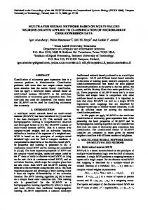
FIGURE 2. Closed loop network application.
The motivation for implementation of a neural network to recover the real process output is to bene®t from the NN’s advantages, such as parallel (i.e. faster) computing, learning capabilities, and generalization properties, (Stephanopoulos and Han 1996, Georgieva and Feyo de Azevedo 2000). The article is organized as follows: in the second section we specify a class of NN able to approximate dynamical models, in the third section we consider two sensor models (without delay and with delay) and their discretization in such a form that their inverses can be approximated by NNs, in the next section the NN architecture and the adaptive algorithm for supervised o -line learning of sensor inverse dynamics are presented. In the following section case-studies for NN compensation scheme are illustrated and the performance of this software mechanism for sensor dynamics compensation is studied in a closed loop operation. The ®nal section addresses a multi-NN structure for improving the robustness of the compensation scheme to changes in the dynamical properties of the measurement system during operation.
NEURAL NETWORK DYNAMICAL STRUCTURE Arti®cial neural networks (ANN) consist of a number of simple interconnected processing units (neurons) and information ¯ow channels between the neurons. The network interconnections have adjustable parameters (weights). During the network training procedure, the interconnection weights are adjusted so that the application of a set of inputs produces the desired set of outputs. A great variety of ANN exist classi®ed by their topology, learning laws, and training algorithms (Kasabov 1996). However, most of the currently used ANN for dynamic modeling and control are layered feedforward neural networks (FNN), also called multi-layer perceptron (Scott and Harmon Ray 1993) and recurrent neural networks (RNN) (You and Nikolaou 1993). A FNN requires as inputs a number of past values for each physical input and output of the dynamical structure (Bhat and McAvoy 1990). The FNN models are de®ned in the discrete time domain with a ®xed sampling period. In a RNN, the outputs of some neurons are fed back to the same neurons or to neurons in preceding layers. Thus, signals can ¯ow in forward and backward directions (Chovan, Catfolis, and Meert 1996).
426
P. Georgieva and S. Feyo de Azevedo
FIGURE 3. O -line FNN training stage.
In this work both feedforward and recurrent neural networks are implemented. A FNN is trained o -line with historical discrete database of sensor input values (arti®cially-generated signals for a certain time period) and sensor output values (recorded response). However, in automatic feedback control systems the sensor inputs are not accessible and therefore, in online application of the trained net, part of the network inputs, corresponding to the sensor inputs, are substituted by past network outputs. Thus, without changing the network topology but changing the network input source we get a RNN. The input-output behavior of a deterministic, time invariant, single-input single-output (SISO) dynamical system can be described by the following discrete time equation: y…k ‡ 1† ˆ f…y…k†; y…k ¡ 1†; . . . ; y…k ¡ n ‡ 1†; u…k† . . . u…k ¡ l ‡ 1††; …1† where the system output at time k ‡ 1 is de®ned by a nonlinear function f…¢† of the past n output values and the past l input values. In practice l is usually smaller than or equal to n. If the function f…¢† is linear, the dynamical system (1) can be represented as: y…k ‡ 1† ˆ a1 y…k† ‡ ...:an y…k ¡ n ‡ 1† ‡ b1 u…k† ‡ b2 u…k ¡ 1† .. . ‡ bl u…k ¡ l ‡ 1† … 2† where ai …i ˆ 1; . . . ; n†; bi …i ˆ 1; . . . ; l† are real constants. When the input-output data and the integers l and n are known, the task of the network is to ®nd a suitable mapping which can approximate function f. It is assumed that systems (1) and (2) are bounded-input bounded-output stable and f does not change with time.
Measurement Dynamics Compensation
427
A straightforward approach to approximate (1) by a network is to choose the input-output structure of the network to be the same as that of the model (1). Hence: yNN …k ‡ 1† ˆ f^…y…k†;y…k ¡ 1†;... ;y…k ¡ n ‡ 1†;u…k†;u…k ¡ 1† ...u…k ¡ l ‡ 1†† … 3† ^ Thus, the network input is transmitted through an activation function f, which has to approximate the function f of model (1). Notice that the network input vector consists of the past system input and output values. A neural network, with input-output relation as in (3), can be easily designed by a three-layered, feedforward network structure with tapped delay of related dimension. The inverse of f…¢† in (1) generates the system input and therefore the inverse dynamical model of the system can be expressed by: u … k† ˆ f
¡1
…y…k ‡ 1†; y…k†; . . . ; y…k ¡ n ‡ 1†; u…k ¡ 1†; . . . ; u…k ¡ l ‡ 1††
… 4†
Then, the input-output relation of a network modeling the inverse dynamical model (4) is: yNN
inv …k†
ˆ f^¡1 …y…k ‡ 1†; y…k†; . . . ; y…k ¡ n ‡ 1†; u…k ¡ 1† . . . u…k ¡ l ‡ 1††
… 5†
There are basically two methods to NN inverse learning: direct inverse learning and specialized inverse learning (see Hunt et al. 1992). These methods are developed in a control context where a NN inverse model of the controlled object is involved to make the system output behave in a desired way. The comparison between the properties of the two inverse learning structures is with respect to the control quality and performance of the closed loop system. In the ®rst method, also referred to as generalized inverse learning, an arti®cial training input signal is supplied to the system. The recorded system output and (arti®cial) system input are then used as input to the network. The error between the network output and the training signal (the system input) is used to train the network. This approach is generally an o -line training procedure and then the ®xed network is placed in a closed loop and used for on-line signal processing. In the second inverse learning method, the network input corresponds to the system reference or command signal. The learning structure includes also a trained (and frozen) forward NN model of the system placed in parallel with the real plant. The di erence between the network input and the
P. Georgieva and S. Feyo de Azevedo
428
forward NN model output (or the plant output) is used as the error signal for the training procedure. The specialized inverse learning is referred as better ``goal directed’’ since it is based on the error between desired system output and actual output. It also overcomes the problem of nonlinear system mapping which is not one-to-one, where the direct inverse learning could produce an incorrect inverse (Hunt et al. 1992). For the present study the direct inverse learning is more suitable, since o -line training with arti®cial training signals seems to be the only possible approach to design a network which approximates inverse measurement dynamics. Moreover, our aim is not process modeling or control and specifying reference or command signals is not a relevant approach.
MODELING OF MEASUREMENT DYNAMICS In control engineering, sensor dynamics is usually represented by a ®rstorder linear time invariant (LTI) model with or without time delay depending on the particular application (Feyo de Azevedo, Oliveira, and Capelo Cardoso 1994). The respective transfer functions are: ym …s† ˆ
km yre …s†; Tm s ‡ 1
… 6†
¡
km e ts ym …s† ˆ yre …s† Tm s ‡ 1
… 7†
where s is Laplace operator, Tm is the time constant, km is the gain and t is the pure time delay between the input yre …¢† considered as the real process output and the measured output ym …¢†. Remark. It has to be emphasized that (6) and (7) do not represent only the dynamics of the measurement device itself (in many cases this is even negligible) but the models include the whole measurement system with additional dynamics due to particular location and conditions of sensor operation. Within the context of a continuous-time system, Pade approximation is commonly used to model time delay e ects as an Nth order polynomial transfer function: e
¡ts
¡ N‡ b1 sN 1 ‡ . . . bN¡1 s ‡ bN ˆs ; ¡ sN ‡ a1 sN 1 ‡ . . . aN¡1 s ‡ aN
Then, substituting (8) in (7) we get:
bi ; ai 2 R;
i ˆ 1; . . . N
… 8†
Measurement Dynamics Compensation
429
…sN ‡ b1 sN¡1 ‡ . . . bN¡1 s ‡ bN † km ym … s † ˆ … yre …s† ¡ Tm s ‡ 1† …sN ‡ a1 sN 1 ‡ . . . aN¡1 s ‡ aN †
… 9†
Considering the network realization we aim for, together with the discrete nature of the measurements, a discrete sensor model becomes the more appropriate to use. Discretization of the continuous model (6) yields the following sensor model: ym …k† ˆ a1 ym …k ¡ 1† ‡ b1 yre …k† ‡ b2 yre …k ¡ 1†;
…10†
and in the same way, the discretized model of (9) is, y m … k† ˆ
‡1 N X i ˆ1
ai ym …k ¡ i† ‡
‡1 N X jˆ 0
bj yre …k ¡ j†
ai ; bj 2 R:
…11†
The inverse measurement dynamics models follow directly from relations (10) and (11), respectively: yre …k† ˆ c1 ym …k† ‡ c2 ym …k ¡ 1† ‡ d1 yre …k ¡ 1†
yre …k† ˆ
N‡ 1 X iˆ 0
ci ym …k ¡ i† ‡
N‡ 1 X jˆ 1
dj yre …k ¡ j†
c1 ; c2 ; d1 2 R;
…12†
ci ; dj 2 R:
…13†
NEURAL NETWORK FOR LEARNING OF INVERSE MEASUREMENT DYNAMICS In this section we consider a feedforward NN as an approximator of measurement inverse dynamics. Although the general FNN is designed to approximate static functions, the parallel network structure where past system input and output enter the network simultaneously introduce dynamic memory, and, in this way, the FNN can approximate mappings of dynamical systems. The network has a ®xed topological structure: one input layer with a dimension that depends on the dimension of the input vector, a single hidden layer, and a linear output layer. The number of neurons and the type of activation function in the hidden layer can be decided according to accuracy requirements of the network approximation. When the measurement dynamics is considered as being linear, only linear activation functions are used in the network model. If, however, the measurement system exhibits a strongly nonlinear behavior, then nonlinear (sigmoidal) activation functions have to be employed.
P. Georgieva and S. Feyo de Azevedo
430
NN Architecture The input-output structure of a FNN able to approximate dynamical models (12) and (13) is the following: yNN …k† ˆ WO F…WI U NN …k††;
…14†
where WI is a matrix of the weights between the input and the hidden layers, WO is a vector of the weights between the hidden and the output layers, and F is a vector of the activation functions in the hidden layer. The network has only one output neuron since at each time there is only one scalar output, yNN …k†. Depending on the sensor model considered, the input vector UNN …k† has di erent dimensions. For sensor dynamics without delay it is: UNN …k† ˆ ‰ ym …k†; ym …k ¡ 1†; yre …k ¡ 1†Š:
…15†
For sensors with ®rst order Pade approximation of the delay the input vector is: UNN …k† ˆ ‰ym …k†; ym …k ¡ 1†; ym …k ¡ 2†; yre …k ¡ 1†; yre …k ¡ 2†Š:
…16†
The higher the order of the delay approximation, the better is the modeling of this nonlinear physical phenomenon, but it leads to enlargement of the network input dimension and for the general case it is: UNN …k† ˆ ‰ym …k†;ym …k ¡ 1†;...;ym …k ¡ N ¡ 1†;yre …k ¡ 1†;. ..;yre …k ¡ N ¡ 1†Š: …17† The motivation for the choice of linear activation functions in the hidden layer is based on the assumption that the measurement device can be considered as having linear or near linear dynamical behavior. In many cases a linear network also may model a nonlinear relationship well enough, provided that enough past signal values are supplied for the network to ®nd the lowest error linear ®t for the nonlinear problem.
TRAINING PROCEDURE The NN is identi®ed o -line using synthetic training inputs. Selected data that cover the normal operating conditions of the sensor is generated. Before starting the training, the weights are initialized with random values between ¡1 and 1. The network is then trained incrementally where the net parameters are updated each time an input vector is supplied to the network. The network is supplied with a training set of desired network behavior:
Measurement Dynamics Compensation
431
fUNN …1†; yT …1†g; . . . ; fUNN …k†; yT …k†g; . . . ; fUNN …l†; yT …l†g; where yT …k† is the scalar target output at time k. The supervised learning procedure is performed with the least mean square error learning rule. The error is calculated as the di erence between the target value and the actual network output. The Widrow-Ho gradient algorithm is applied to adjust the network parameters. They are moved in the direction of the negative gradient of the performance function (Widrow and Ho 1960).
Validation Stage After the training is complete we simulate the network response with new ``unseen’’ data to test the quality of the training. At each time the network computes its estimate of the real output (by Equation (17)) but with a new structure of the input vector: For sensor dynamics without delay: UNN …k† ˆ ‰ym …k†; ym …k ¡ 1†; yNN …k ¡ 1†Š
…21†
and, for sensor dynamics with ®rst-order Pade approximation of the delay: UNN …k† ˆ ‰ym …k†; ym …k ¡ 1†; ym …k ¡ 2†; yNN …k ¡ 1†; yNN …k ¡ 2†Š
…22†
It should be noted that at this stage the past values of the sensor input are substituted by the previous values of the network output. In contrast to the training stage where FNN are implemented, at the validation stage the network has a recurrent structure (see Figure 4). The reason for involving a feedback in the network is that this is the actual way of network operation in a closed loop system. The sensor inputs are not accessible and we assume that the trained network gives reliable estimates. The procedure can thus be summarized as follows:
FIGURE 4. O -line RNN validation stage.
P. Georgieva and S. Feyo de Azevedo
432
a) b) c) d) e)
Generate input data (arti®cial `real process outputs’) for the sensor Store the sensor responses (measured outputs) Initialize the network architecture (number of inputs, activation function) Assign initial (random) values to all network parameters Implement incremental training procedure 1. Supply the appropriate input patterns and calculate the network output and error 2. Update the parameters with adaptive learning rate. f) Proceed with validation stage (NN simulation with new input data)
SIMULATION STUDIES In this section the procedure for measurement dynamics compensation described in the previous sections is illustrated with simulations. Several sequences of sensor input signals (representing `real process outputs’) were generated under the mild restriction that they had to be positive-bounded functions in a pre-speci®ed time interval. Table 1 lists this set of generated signals, which were also used as the target sequences for the supervised incremental network training. They were generated for a time horizon of 10 min with a sampling rate of 20 samples per minute. Their trajectories vary from a pure step, through step-like, ramp, and sine shape. Some of the signals were designed as a mixture of di erent shapes so that di erent sensor transient behaviors were excited. The time responses of the sensor (the measured outputs) to the input signals of Table 1 were stored as time series. The network has one hidden layer with two linear activation functions. The initial learning rate, in all subsequent experiments, was set to 0.5.
First Order Measurement Dynamics Without Delay In the ®rst study, the measurement dynamics model (represented by Equation 6) was considered with parameters Tm ˆ 0.5 min, km ˆ 1. The TABLE 1 Signal generation for `real process outputs’ Signals
Signals
A
yre …t† ˆ 0:3t; t 2 ‰0; 10 Š
B
C
yre …t† ˆ 1:5; t 2 ‰0; 10 Š 8 2‰ Š > > < 0:5 t 0; 3 2 …3; 5Š 1 t yre …t† ˆ > 2 …5; 8Š > : 1:5 t 0:8 t 2 …8; 10 Š
D
G
F
yre …t† ˆ 1:5 ‡ sin …t†; t 2 ‰0; 10Š 8 < 0:5 ‡ 0:3t; t 2 ‰0; 3:3Š yre …t† ˆ : yre …t ˆ 3:3†; t 2 …3:3; 6:7Š 1:5 ‡ 0:5 sin…1:5t†; t 2 …6:7; 10Š 8 < 1 ‡ 0:5 sin 1:5t t 2 ‰0; 3:3Š yre …t† ˆ : 0:5 t 2 …3:3; 6:7Š 0:5t t 2 …6:7; 10 Š
Measurement Dynamics Compensation
433
results are summarized in Figure 5 and Figure 6. Figure 5a (upper left plot) shows the network training stage with a ramp signal (A) as real process output (RPO). The measured output (MO) di ers from the real process output. The solid line on Figure 5a shows the NN output (NNO) obtained after the adaptation procedure. It matches up perfectly with the target and the error (E) is zero. The other plots in the same ®gure present the validation stage, when the parameters of the NN were ®xed and the network was tested applying di erent target sequences ± i) the real process output (RPO) as a sine signal (Figure 5b); ii) RPO as a step=like signal (Figure 5c); and iii) RPO as a more complex time function (Figure 5d). This study addresses also the nature of the training signal and con®rms that this is of crucial importance. The comparison between the generated training signals leads to the conclusion that they have to be faster than the sensor dynamics so that they persistently excite its transient behavior
FIGURE 5. NN training and validation for case study 5.1. a) training with signal A; b) validation with signal B; c) validation with signal G; d) validation with signal D. NN output (NNO), real process output (RPO), measured output (MO), error (E).
434
P. Georgieva and S. Feyo de Azevedo
(Rovithakis and Christodoulou 1995). Also, the training signals have to cover the range of expected operational signals. When a constant signal was applied as training sequence the network failed to work properly and did not recover new target signals. The best tracking was achieved for the steep ramp function. Two training procedures are depicted in Figure 6. Both of them were performed with step-like target signals, but the second one (plot c) with ten times larger step levels. The two networks were then validated with a sine target signal, which was in the same range of the ®rst training signal (plot a) but far away from the second training signal (plot c). The ®rst network recovers well new data (plot b) whereas the second network fails to recover new signals (plot d).
First Order Measurement Dynamics with Delay The results for training a NN to approximate the inverse of the measurement dynamics model (7) are summarized in Figure 7 and Figure 8. The
FIGURE 6. NN training and validation for case study 5.1. a) training with signal G; b) validation with signal B; c) training with 10*G; d) validation with signal B. NN output (NNO), real process output (RPO), measured output (MO), error (E).
Measurement Dynamics Compensation
435
sensor parameters were set to Tm ˆ 0.5 min, km ˆ 1, and t ˆ 0.4 min. The upper left plot (a) on Figure 7 shows the training stage when the real process output (RPO) is a ramp function. The other plots in the same ®gure (b, c, and d) show a good network performance when tested with new data. However, the tracking deteriorated slightly within the delay period when some rapid changes occurred in the target signal. As in the previous case, the nature of the training signal appears to be of great importance. For constant signal the network was not able to learn the sensor inverse dynamics. Figure 8 depicts the same training signals (step-like and step-like with ten times larger step levels) and the same validation signal (B) as those reported in Figure 6, now applied to the sensor dynamics with delay. The results con®rm the inability of the network to react properly to new signals external to the operational training signal range. Remark. A general question can be raised about the type of data employed for NN training. This should not be performed with occasional or
FIGURE 7. NN training and validation for case study 5.2. a) training with signal A; b) validation with signal B; c) validation with signal G; d) validation with signal D. NN output (NNO), real process output (RPO), measured output (MO), error (E).
436
P. Georgieva and S. Feyo de Azevedo
FIGURE 8. NN training and validation for case study 5.2. a) training with signal G; b) validation with signal B; c) training with 10*G; d) validation with signal B. NN output (NNO), real process output (RPO), measured output (MO), error (E).
randomly-chosen signals. For investigating the ability of a NN to identify inverse measurement dynamics in general, it is required to select persistentlyexciting signals faster than the sensor dynamics. Therefore, network training with properly-generated signals, which cover the sensor operational range, is more appropriate than using actual process data.
Closed Loop Network Application The e ciency of the NN-based measurement dynamics compensation was studied in terms of its e ects in the performance of a closed loop control system. We considered a simple illustrative example where the process dynamics was assumed to be well approximated by a ®rst-order model, with a transfer kp function yre …s† ˆ T ps ‡1 u…s†: kp and Tp are the process gain and time constant, respectively. A proportional controller (with a gain kreg ) was designed so that
Measurement Dynamics Compensation
437
it guaranteed stability of the closed loop system and a steady-state tracking error up to 1%. A measurement dynamics, represented by Equation 7, was considered in the study. The system parameters, for which the simulations were performed, were set to be kreg ˆ 7:5; kp ˆ 1:2; km ˆ 1; Tp ˆ 1:5; Tm ˆ 0:15; and t ˆ 0.075. The network was ®rst trained o -line and then the ®xed network was placed in closed loop, as shown in Figure 9. The closed loop system behavior was studied with respect to two di erent time varying reference signals: step-like and sine-shaped (depicted in Figure 10). In a ®rst instance the output time trajectory of the closed loop system without the NN structure was simulated (marked in Figure 10 by MO-measured output). Then the closed loop system was simulated with the NN compensator in operation, i.e. with the controller receiving process information from the NN output (e…k† ˆ r…k† ¡ yNN …k†). Figure 10 presents information concerning two relevant aspects of this study, viz. ± (i) it shows that the neural network output (NNO) matches very well the real process output (RPO), i.e., that the compensator works well in this closed loop test; and (ii) it shows that with the compensator, the closed loop transient performance has improved.
MULTI-NN RECOVERING SYSTEM As noted in the preceding sections, the single NN structure for measurement dynamics compensation is only able to recover su ciently well the real output in those cases where the real sensor does not di er considerably from the sensor model used at the o -line training stage or where data from the real sensor is used for o -line training. In this statement it is implied that the quality of signal recovering is strongly a ected by any changes which may occur in the sensor behavior (represented by parameters ± time constant or delay) during its operational life. Our tests have shown that the recovering deteriorated rapidly when the time constant di ered by more than 4% from the time constant employed for training.
FIGURE 9. On-line closed loop NN sensor dynamics compensation.
438
P. Georgieva and S. Feyo de Azevedo
FIGURE 10. Closed loop output trajectory. a) step-like reference signal (ref); b) sine reference signal (ref) NN output (NNO), real process output (RPO), measured output (MO), error (E).
To overcome this real problem and to make the network more e cient for applications, a multiple concurrent-network recovering system has been developed. This includes a step of periodical calibration, which consists, in fact, of a periodical choice of the optimal network path for output recovering. The multiple network structure is represented in Figure 11. Firstly, a sensor model is identi®ed and one network is o -line trained with this model that is assumed to represent the sensor dynamics su ciently well. We consider this as a nominal sensor model and the respective network as a nominal network. Then, several networks are o -line trained for sensor models with di erent parameters, covering a range of expected changes. This multi-NN structure, including n trained networks, is placed in series with the sensor in the closed loop system. From all outputs, produced by the network, only one will be active, supplying the controller input during actual operation. The active path is selected by the periodical calibration procedure, being kept the same between calibrations.
Measurement Dynamics Compensation
439
FIGURE 11. Multi-NN recovering system.
The Calibration Procedure During calibration all paths are active. Each network receives the sensor output and produces an element of the network output vector YNN …k† ˆ ‰yNN1 …k†; yNN2 …k†; . . . ; yNNn …k†Š. The scalar output of the system, y^re …k†, that will supply the controller with the process output data, is chosen to be this output of the multi-network structure that has a minimal distance to the process output signal yre , corresponding to y^re …k† ˆ fyNNj …k† : minjˆ1¥n jyre …k† ¡ yNNj …k†jg The calibration requires manual measurements of the real output. This is one of the reasons why the calibration cannot be performed continuously. Moreover, too frequent calibrations would cause output oscillations due to the switching e ect between the di erent pathways. Therefore, it is recommended the calibration to be carried out periodically (once a day or once a week) depending on how often signi®cant changes in the sensor parameters are expected to occur. The simulation results in Figure 12 are performed with ®ve networks trained for the nominal and four other sensor models with 10% and 20% variation around the nominal parameters (see Table 2). The multi-neuron network structure consists of all trained networks. The same illustrative example as in the subsection on closed loop network application is considered, but with the multi-NN structure placed in series with the sensor. The closed loop system is ®rst simulated with the nominal sensor model, (Figure 12a). Hence there exists a NN that is trained for this sensor and it is not strange that the network output (NNO) recovers with a high precision the real process output (RPO). The measured output (MO) is also depicted on the same plot. On the next plot (Figure 12b) the same signals are shown for a process run with sensor parameters that di er from those used for training but
440
P. Georgieva and S. Feyo de Azevedo
nevertheless in the range of expected variations (Table 2). The recovering is almost not a ected although the time constant and the delay are changed. The switching e ect between the network outputs appears only slightly in the plot. If more networks are trained, the real output recovering will be even better, but network output oscillations may be observed. Therefore, assuming that the sensor does not change its parameters very frequently, the calibration should be performed only periodically and for a limited multi-NN structure. A main advantage of this signal recovering structure is that it is simple in its design and does not require a lot of computational power. It is based on the assumption that the measuring dynamics belong to a certain class (Equations (6) and (7)) with parameters that are assumed to vary within known bounds and a calibration can be regularly performed. If these assumptions cannot be veri®ed, then a sound alternative for switching between di erent network models would be to apply some sort of pattern recognition technique, though this is known to require more data and computational sources.
FIGURE 12. Closed loop output trajectory with multi-NN structure. a) Sensor with nominal parameters Tm ˆ 0:15; t ˆ 0:075; b) Sensor with parameters Tm ˆ 0:1725; t ˆ 0:065. NN output (NNO), real process output (RPO), measured output (MO).
Measurement Dynamics Compensation
441
TABLE 2 Sensor parameter variation Sensor Param. Tm [min] t [min]
Nominal NN
NN1 ( ‡ 20%)
0.15 0.075
0.18 0.09
NN2 ( ‡ 10%)
NN3 ( ¡10%)
0.165 0.0825
0.135 0.0675
NN4 (¡20%)
Real sensor
0.12 0.06
0.1725 0.065
CONCLUSIONS NN-based structure has been presented for the recovering of process outputs from sensor signals. The network topology was speci®ed as a tree-layered net with backpropagation training algorithm and adaptive learning rate. The following basic requirements for reliable output recovering were established: ° The network training is either performed with a sensor model which describes the real sensor su ciently well or directly with the real measurement device. Whatever the case, it is required to generate input data to the sensor, get its time responses, and provide the network with the training data. ° The training signals have to be faster than the sensor dynamics so that they persistently excite its dynamics. At the same time they have to cover the space of the expected operational signals. ° Also, there is no need for a too-long training time series. In average, the adaptation converges after 10±15 iterations. It has been shown that it is possible to develop NN compensators that provide very accurate recovering of data distorted by ®rst-order dynamics, including time delays. The solution proposed may improve the performance of closed-loop control systems in those cases where measurement signals are a ected or di er from the real process outputs by the above cited dynamics. In real-time applications, sensor dynamics characteristics may change along its operational life. This may lead to wrong estimates when employing a NN trained for the original sensor parameters. An e cient solution to this problem is the use of a multi-NN structure for signal recovering system, as presented in the paper. Further research will be carried out aiming at the study of the recovering ability and robustness properties of the network in the presence of measurement noise.
REFERENCES Bhat, N., and T. J. McAvoy. 1990. Use of neural nets for dynamic modelling and control of chemical process systems. Computers Chem. Engng. 14(4=5):573±583. Cheng, Y., T. W. Karjala, and D. M. Himmelblau. 1995. Identi®cation of nonlinear dynamic processes with unknown and variable dead time using an internal recurrent neural network. Ind. Eng. Chem. Res. 34(5):1735 ±1742.
442
P. Georgieva and S. Feyo de Azevedo
Chovan, T., T. Catfolis, and K. Meert. 1996. Neural network architecture for process control based on the RTRL algorithm. AIChE Journal 42(2):493±502. Chtourou, M., K. Najim, G. Roux, and B. Dahhou. 1993. Control of a bioreactor using a neural network. Bioprocess Engineering 8:251±254. Feyo de Azevedo, S., B. Dham, and F. Oliveira. 1997. Hybrid modelling of biochemical processes: A comparison with the conventional approach, Computers Chem. Engng. 21 (Suppl.): S751±S756. Feyo de Azevedo, S., F. Oliveira, and A. Capelo Cardoso. 1994. TEACON-a simulator for computeraided teaching of process control. Computer Applications in Engineering Education 1(4):307±319. Georgieva, P., and S. Feyo de Azevedo. 2000. Measurement dynamics compensation using neural network inverse modelling. Proc. of 4th Portuguese Conference on Automatic Control CONTROLO’2000, 318±323. GuimaraÄes, Portugal, October 4±6, 2000. Glassey, J., M. Ignova, A. C. Ward, G. A. Montague, and A. J. Morris. 1997. Bioprocess supervision: Neural networks and knowledge based systems. Journal of Biotechnology 52:201±205. Hunt, K. J., D. Sbarbaro, R. Zbikowski, and P. J. Gawthrop. 1992. Neural networks for control systems a survey. Automatica 28(6):1083±1112. Kasabov, N. 1996. Foundations of Neural Networks, Fuzzy Systems and Knowledge Engineering. Cambridge, MA: MIT Press. Nahas, E. P., M. A. Henson, and D. E. Seborg. 1992. Nonlinear internal model control strategy for neural network models, Computers Chem. Engng. 16(12):1039±1057. Narendra, K. S. 1990. Neural networks for control. Cambridge, MA: MIT Press. Narendra, K. S., and K. Parthasarathy. 1990. Identi®cation and control for dynamical systems using neural networks. IEEE Trans. On Neural Networks 1:4±27. Pham, D. T., and X. Liu. 1995. Neural Networks for Identi®cation, Prediction and Control. London: Springer Verlag. Rovithakis, G. A., and M. A. Christodoulou. 1995. Direct adaptive regulation of unknown nonlinear dynamical systems via dynamic neural networks. IEEE Trans. On Systems, Man and Cybernetics 25(12):1578±1594. Schubert, J., R. Simutis, M. Dors, I. Havlik, and A. LuÈbbert. 1994. Bioprocess optimisation and control: application of hybrid modelling. Journal of Biotechnology 35:51±68. Scott, G. M., and W. Harmon Ray. 1993. Creating e cient nonlinear neural network process models that allow model interpretation. Journal of Process Control 3(3):163±178. Simutis, R., R. Oliveira, M. Manikowski, S. Feyo de Azevedo, and A. LuÈbbert. 1997. How to increase the performance of models for process optimization and control. Journal of Biotechnology 59:73±89. Stephanopoulos, G., and Ch. Han (Eds.) 1996. Intelligent Systems in Process Engineering. London, UK: Academic Press. Tham, M. T., A. J. Morris, and G. A. Montague. 1989. Soft-sensing: a solution to the problem of measurement delays. Che. Eng. Res. Des. 67:547±554. Widrow, B., and M. E. Ho . 1960. Adaptive switching circuits. IRE WESCON Convention record, New York, 96±104. Yesildirek, A., and F. L. Lewis, 1995. Feedback linearization using neural networks. Automatica 31(11):1659±1664. You, Y., and M. Nikolaou. 1993. Dynamic process modelling with recurrent neural networks, AIChE Journal 39(10):1654±1667.