Warsaw University of. Technology. Pl. Politechniki 1. 00-661 Warsaw, Poland. Tomasz ..... following the previous convention, we denote the number of paths.
A New Approach to Betweenness Centrality Based on the Shapley Value ∗
´ Piotr L. Szczepanski
Tomasz Michalak
Talal Rahwan
Institute of Informatics, Warsaw University of Technology Pl. Politechniki 1 00-661 Warsaw, Poland
Institute of Informatics, University of Warsaw 02-097 Warsaw ul. Banacha 2, Poland
Electronics and Computer Science, University of Southampton SO17 1BJ University Road, UK
ABSTRACT
Categories and Subject Descriptors
In many real-life networks, such as urban structures, protein interactions and social networks, one of the key issues is to measure the centrality of nodes, i.e. to determine which nodes and edges are more central to the functioning of the entire network than others. In this paper we focus on betweenness centrality — a metric based on which the centrality of a node is related to the number of shortest paths that pass through that node. This metric has been shown to be well suited for many, often complex, networks. In its standard form, the betweenness centrality, just like other centrality metrics, evaluates nodes based on their individual contributions to the functioning of the network. For instance, the importance of an intersection in a road network can be computed as the difference between the full capacity of this network and its capacity when the intersection is completely shut down. However, as recently argued in the literature, such an approach is inadequate for many real-life applications, as, for example, multiple nodes can fail simultaneously. Thus, what would be desirable is to refine the existing centrality metrics such that they take into account not only the functioning of nodes as individual entities but also as members of groups of nodes. One recently-proposed way of doing this is based on the Shapley Value — a solution concept in cooperative game theory that measures in a fair way the contributions of players to all the coalitions that they could possibly participate in. Although this approach has been used to extend various centrality metrics, such an extension to betweenness centrality is yet to be developed. The main challenge when developing such a refinement is to tackle the computational complexity; the Shapley Value generally requires an exponential number of operations, making its use limited to a small number of player (or nodes in our context). Against this background, our main contribution in this paper is to refine the betweenness centrality metric based on the Shapley Value: we develop an algorithm for computing this new metric, and show that it has the same complexity as the best known algorithm due to Brandes [7] to compute the standard betweenness centrality (i.e., polynomial in the size of the network). Finally, we show that our results can be extended to another important centrality metric called stress centrality.
H.4 [Information Systems Applications]: Miscellaneous ; D.2.8 [Software Engineering]: Metrics—complexity measures, performance measures
General Terms Algorithms, Graph Theory, Game Theory
Keywords Betweenness Centrality, Shapley Value
1.
INTRODUCTION
Appears in: Proceedings of the 11th International Conference on Autonomous Agents and Multiagent Systems (AAMAS 2012), Conitzer, Winikoff, Padgham, and van der Hoek
Networks (or graphs) are a very natural representation of a variety of real-life domains such as, among others, urban structures [20], protein interactions [6], social networks [25] and computer communication networks [13, 27]. Networks are also an important modeling paradigm in Multi-Agent System (see, e.g., [2, 11]). In many of these applications, it is often paramount to determine which nodes (or vertices) and edges are more critical (or central) to the functioning of the entire network than others. For example, one may need to know the most influential persons in a social network or the most important routes in a road network. To this end, various centrality metrics, such as degree, closeness, eigenvalue or betweenness, have been extensively studied in the literature.1 In this paper we focus on betweenness centrality — a metric based on which the centrality of a node is related to the number of shortest paths that pass through that node. The importance of this centrality metric stems from the fact that it characterizes well many, often complex and extensive, networks. In particular, a variety of naturally evolving real-life networks, such as the internet or social networks, feature a power-law distribution of betweenness centrality (as well as degree centrality) [3, 13]. Intuitively, in these so called scale-free networks, there are relatively few nodes that contribute to a large number of shortest paths. This implies that such networks are hardly affected by random impairments but, at the same time, they can be relatively easily affected by the removal of the most central nodes [4]. For example, it was shown in the epidemiology literature that the immunization of the most central nodes significantly hinders epidemics [19]. As another example, in the internet context, the betweenness centrality can be used to identify nodes in a local network that are able to trace the communications of as many users as possible [21].
(eds.), 4-8 June 2012, Valencia, Spain. c 2012, International Foundation for Autonomous Agents and Copyright Multiagent Systems (www.ifaamas.org). All rights reserved.
1 An overview of the most important centrality metrics can be found in Koschützki at al. [18].
∗
The authors would like to thank all four anonymous reviewers for their useful comments that significantly improved the paper.
Due to a variety of important applications, an ongoing line of research tries to develop better centrality metrics that are more suitable for diverse real world situations [14]. Consider, for example, the problem of designing an infrastructure network, such as a communication network or power grid, where the design is required to be resistant to random node failures. In this respect, centrality metrics, which in this case are called vitality measures [18], simply test the performance of a network with and without a given node. For instance, the importance of an intersection in a road network can be computed as the difference between the full capacity of this network and its capacity when the intersection is completely shut down. Naturally, the more adverse the consequences of a node failure are, the higher the centrality of this node becomes. Nevertheless, such an approach to computing centrality is often inadequate for many real-life network applications.2 In more detail [1]: • It is often insufficient to merely consider failures of individual nodes. This is because, in many real-world situations, multiple nodes can fail simultaneously. This was, for instance, the case with the Japanese power grids that were destroyed during the 2011 tsunami. Whereas not much capacity is lost when individual nodes fail in such a network, multiple concurrent failures of certain critical nodes can be highly detrimental. Such issues, however, are not considered in the standard centrality metrics; • A related impediment of standard centrality metrics is the implicit assumption of node failure independence. This assumption does not hold in many real-world situations when nodes break down sequentially in a short period of time [26]. In an attempt to address the above shortcomings, the notion of group centrality [12] has been proposed by which centrality is measured not only for individual nodes but also for groups of them. Whereas, in principle, this notion tackles the issue of group failures, its use is rather limited. This is because it only answers the question of how important a certain group of nodes is. However, it is often unknown ex ante which particular groups of nodes should be considered, e.g., in a natural disaster scenario, where it is not possible to identify a priori the nodes that will be affected. Even if we evaluate all possible groups, we are still left without a synthetic ranking of individual nodes’ importance. Thus, what would be more desirable is to have a metric of importance of an individual node that takes into account many (preferably all) potential groups that this node can belong to. One such metric is the recentlyproposed notion of the game theoretic network centrality [15, 24] based on the Shapley Value. In more detail, the Shapley Value is one of the key solution concepts in game theory. It advocates a fair division of payoff from a coalitional game and is computed as the weighted average of marginal contributions of players to all the coalitions that they could potentially participate in. The basic idea behind the Shapley Value-based centrality is to define a game over the network, where nodes are players and collections of nodes are coalitions. In this game, the value of any coalition reflects the consequences of a simultaneous failure of all the nodes involved in this coalition. The marginal contribution of a node to a coalition is interpreted as the change in severity of such a failure if this additional node failed with all the other nodes already involved in the coalition. The Shapley Value computed for such a game shows the weighted average of all the marginal contributions of each node to all the potential coalitions of nodes. This addresses both problems related to the standard centrality metrics. Note, however, that 2 A failure of a node should be understood as an inability to perform its previous role, e.g. to control the information flow.
computing the Shapley Value in the general case requires a number of operations that is exponential in the number of players. This is clearly not desirable, especially given networks with large numbers of nodes. Thus, to be able to use Shapley Value-based metrics in practice, it is crucial that this complexity is significantly reduced. Against this background, our contributions in the present paper can be summarised as follows: 1. To date, the Shapley Value was used to refine two standard metrics: degree centrality [24] and closeness centrality [1]. Our first contribution in this paper is to develop the refinement of the betweenness centrality metric based on the Shapley Value; 2. We propose a polynomial-time algorithm for computing the new metric. Interestingly, although our algorithm involves the computation of the Shapley Value, we show that it has the same complexity as the best known algorithm due to Brandes [7] to compute the standard betweenness centrality. 3. Finally, we show that the above results can be extended to another centrality metric, namely the stress centrality [23, 18] — a concept closely related to betweenness centrality. The remainder of the paper is organized as follows. In Section 2, basic notations and definitions are presented. In Section 3, we introduce the new betweenness centrality based on the Shapley Value. The polynomial time algorithm to compute the new metric is described in Section 4. In Section 5, we summarize our results and present the most promising directions for future research. Finally, a proof is provided in the appendix.
2.
PRELIMINARIES
In this section we introduce basic concepts from cooperative game theory that are needed in our analysis. A graph (or network) G is composed of vertices (or nodes) and edges. Their sets will be denoted V (G) and E(G), respectively, where every edge in E(G) connects two vertices in V (G). An edge connecting vertices u, v ∈ V (G) will be denoted by (u, v). We will also consider weighted networks in which a weight (label) is associated with every edge in E(G). Informally, a path is a sequence of connected edges. The shortest path between two given vertices u and v is a path that ends with these vertices and minimizes the weights of the involved edges (or minimizes the number of edges in the case of unweighted networks). It will be denoted by p u ; v or simply p if there is no risk of confusion. Next, we define the notion of a coalitional game and the Shapley Value [22]. In particular, by A = {a1 , . . . , a|A| } we will denote the set of players that participate in a coalitional game. A characteristic function ν : 2A → R assigns to every coalition C ⊆ A a numerical value representing its performance. It is assumed that ν(∅) = 0. A coalitional game in a characteristic function form is then a tuple (A, ν). It is usually assumed that the grand coalition, i.e. the coalition of all the players in the game, has the highest value and, therefore, is formed. One of the fundamental questions in cooperative game theory is how to divide the payoff from the grand coalition between the players. Whereas, in principle, there may be an infinite number of such divisions, we are interested in those that meet certain desirable criteria. In this respect, in his highly-regarded paper, Shapley proposed to evaluate the role of each player in the game proportionally to a (weighted) average marginal contribution of this player to all possible coalitions. The importance of the Shapley Value stems from the fact that it is the
unique division scheme that meets the following four fairness criteria: 1. Efficiency — the entire payoff of the grand coalitions is distributed among players; 2. Symmetry — all players with the same marginal contributions to all coalitions receive exactly the same payoff; 3. Null player — players with no marginal contribution to every coalition receive no payoff; and 4. Additivity — values for two given games sum up to the value computed for the sum of both games. To formalize this concept we denote by π ∈ Π(A) a permutation of players in A, and by Pπ (i) the coalition made of all predecessors of player ai in π. In more detail, denoting by π(j) the location of aj in π, we have Pπ (i) = {aj ∈ π : π(j) < π(i)}. Shapley [22] defined the value of ai , denoted SVi (A, ν), as the average marginal contribution of ai to coalition Pπ (i) over all π ∈ Π. Formally: 1 X SVi (A, ν) = [ν(Pπ (i) ∪ {ai }) − ν(Pπ (i))]. (1) |A|! π∈Π The intuition behind the above formula is as follows: suppose that the players arrive at a certain meeting point in a random order. Furthermore, assume that every player ai who arrives receives the marginal contribution that this arrival brings to those already at the meeting point. The payoff of player ai from the coalitional game is then the average of these contributions taken over all the possible orders of arrival. The above formula can be rewritten into an equivalent form as: X |S|!(|A| − |S| − 1)! [ν(S ∪ {ai }) − ν(S)]. (2) SVi (A, ν) = |A|! S⊆A\{ai }
In the network context, we will denote a coalitional game defined on network G by (V (G), ν), where a set of vertices is a set of players, A = V (G), and ν : 2V (G) → R is the characteristic function, where ν(∅) = 0. Sometimes, we will use the phrase “value of coalition S” when referring to ν(S).
3.
SHAPLEY VALUE-BASED BETWEENNESS CENTRALITY
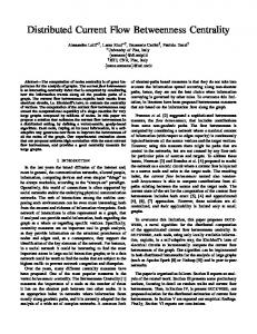
In this section we propose the Shapley Value-based betweenness centrality. We start with the definition of the standard betweenness centrality [14]: Definition 1. The betweenness centrality of a vertex v is defined P (v) 3 as a function c : V → R : cb (v) = s6=v6=t σst , where σst is σst the number of shortest paths from s to t (if s = t then σst = 1), and σst (v) is the number of shortest paths from s to t passing through vertex v (if v ∈ {s, t} then σst (v) = 0). Intuitively, the betweenness centrality metric represents the load placed on a given vertex in a network. One of the key applications of this metric is to measure the ability of different nodes to control the information flow within a network. However, as we will now show, there are cases where the standard betweenness centrality metric does not produce accurate measurements in such applications. Consider, for example, the network in Figure 1. By computing the centrality of each node in this network using the standard 3
To deal with unconnected graphs it is assumed that
0 0
= 0.
Figure 1: Sample network. betweenness metric, we find that both v9 and v10 are ranked equally (i.e., cb (v9 ) = cb (v10 ) = 98)! This is clearly not accurate since the failure of v9 has more adverse consequences on the ability to pass information through the network than the failure of v10 . For example, if v10 fails, then the bottom right nodes (i.e., v16 , v17 , v18 , and v19 ) can still communicate with one another. On the other hand, if v9 fails, then the bottom left nodes (v12 , v13 , v14 , and v15 ) can no longer communicate with each other. In an attempt to deal with this issue, Everett and Borgatti [12] proposed the notion of group betweenness centrality of the form: X σst (S) , cgb (S) = σst s∈S / t∈S /
where S ⊆ V (G) is a subset of vertices under consideration, and σst (S) is the number of the shortest paths from s to t passing through some vertex in S (if s ∈ S or t ∈ S then σst (S) = 0). This centrality metric, however, only evaluates a given subset of vertices S, and this implies that the evaluation of individual nodes remains unchanged. For instance, given the network in Figure 1, group betweenness centrality gives exactly the same ranking of v9 and v10 as the standard betweenness centrality, i.e., cgb (v9 ) = cgb (v10 ) = 98 (the only difference is that the former centrality evaluates {v9 } and {v10 }, while the latter one evaluates v9 and v10 , respectively; this change does not affect the evaluations of those two nodes). Therefore, even if we evaluate all possible 2|V (G)| subsets using group centrality, we are still left without one synthetic ranking of individual vertices’ importance. To address this problem, we now introduce the Shapley Valuebased betweenness centrality: Definition 2. Given a network G, the Shapley Value-based betweenness centrality of a vertex v ∈ V (G) is defined as a function cSh : V → R : cSh (v) = SVv (V (G), ν), where ν is the characP σst (S) teristic function defined as ν : 2V (G) → R : ν(S) = s∈S / σst t∈S /
with S ⊆ V (G). As mentioned in Section 2, the Shapley Value divides the payoff of the grand coalition among players by evaluating their marginal contributions to any coalition they may possibly belong to. Simply, the higher these marginal contributions are, the higher the Shapley value of a player is. Or, to rephrase it in the context of this paper, the more a vertex contributes to the performance of any possible group of vertices (that this vertex belongs to), the higher
its betweenness centrality should be. Thus, unlike the group betweenness centrality, our Shapley Value-based centrality provides synthetic ranking of individual vertices’ importance. Coming back to the example in Figure 1, we find that: cSh (v9 ) = 18.2, while cSh (v10 ) = 16.0833. In other words, our metric is able to reflect the difference in centrality between v9 and v10 because the evaluation of each node is done from a global perspective of all subsets in the network. This approach, among other advantages, grasps a nuance that {a10 , a11 } play the the same role as {v9 }, and this because cgb ({v9 }) = cgb ({v10 , v11 }). Our notion can be seen as analogous to the Shapley Value-based degree and closeness centralities. Having defined it, in the next section we will propose a polynomial time algorithm to compute it.
4.
ALGORITHMS TO COMPUTE THE SHAPLEY VALUE BASED BETWEENNESS CENTRALITY
Although the formula for the Shapley Value in (2) is less computationally involved than in (1), it still requires analyzing a number of coalitions that is exponential in the number of players. Specifically, in our network context one would need to analyse O(2|V (G)| ) coalitions, i.e., groups, of vertices. To circumvent this major obstacle, we propose in this section two polynomial algorithms for computing the Shapley Value-based betweenness centrality: one for weighted graphs, and the other for unweighted graphs. Interestingly, we show that the first algorithm has the same complexity as the best known algorithm to compute the betweenness centrality in the standard form (due to Brandes [7]). Furthermore our both algorithms can be easily adapted to work on directed graphs.
4.1
A Look at Marginal Contributions
Given a graph G and some vertex v ∈ V (G), we would like to compute the expected marginal contribution of this vertex to the set of vertices Pπ (v) occurring before v in a random permutation π of all vertices of the graph. We split our analysis into two cases: one of positive and one of negative marginal contributions, respectively. Firstly, we consider positive contributions. In what follows, let us focus on some particular shortest path p which contains vertex v. Recall that we denote by σst the number of shortest paths between vertices s and t, and by σst (v) the number of shortest paths between vertices s and t where every path passes through vertex v and v 6= t 6= s. Every path in σst (v) has a positive contribution to the coalition Pπ (v) through v if and only if it is not yet controlled by any vertex from set Pπ (v). In this case, the positive contribution equals σ1st . The necessary and sufficient condition for this to happen can be expressed by Ψ(p) ∩ Pπ (v) = ∅, where Ψ(p) is the set of all vertices lying on the path p including endpoints. That is, vertices s and t, as well as the rest of the vertices from path p, should not belong to Pπ (v). + Now, let us introduce a Bernoulli random variable Bv,p which indicates whether vertex v makes a positive contribution through path p to set Pπ (v). Thus, we have: 1 1 + Bv,p ] = P [Ψ(p) ∩ Pπ (v) = ∅], E[ σst σst where P [·] denotes probability, and E[·] denotes expected value. In other words, we need to know the probability of having v precede all other vertices from Ψ(p) \ {v} in a random permutation of all vertices in the graph. Combinatorial arguments (see the Appendix) 1 show that this happens with probability |Ψ(p)| . Thus: E[
1 + 1 Bv,p ] = . σst σst |Ψ(p)|
(3)
Secondly we examine a potential negative contribution of vertex v to set Pπ (v). Such a contribution happens when path p ends with v. Specifically, if coalition Pπ (v) already controls path p, along with vertex v, then not only is there no value added from v becoming a member of this coalition, but there is a negative effect of this move. In particular, the group betweenness centrality assumes that a set of vertices S controls only those paths with both ends not belonging to S. Therefore, when v becomes a member of coalition Pπ (v), its negative contribution through path p is − σ1sv , where, following the previous convention, we denote the number of paths that start with some s end with v by σsv . Now, we will analyse a probability of such a negative contribution to happen by considering a complementary event in which path p makes neutral contribution to set Pπ (v). This happens if and only if either vertex s belongs to set Pπ (v), or this path is not controlled by any of the vertices in Pπ (v). Formally: s ∈ Pπ (v) ∨ (Ψ(p) ∩ Pπ (v)) = ∅. Now, by introducing a Bernoulli − random variable Bv,p which indicates whether that vertex v makes a negative contribution through path p to set Pπ (v), we get the following expression: E[−
1 1 − Bv,p ] = − (1−P [s ∈ Pπ (v)∨(Ψ(p)∩Pπ (v)) = ∅]). σsv σsv
Again, one can show with combinatorial arguments that this prob1 ability is P [Ψ(p) ∩ Pπ (v) = ∅] = |Ψ(p)| and due to symmetry that 1 P [s ∈ Pπ (v)] = 2 . Finally, from the disjointness of these two events, we
E[−
2 − |Ψ(p)| 1 − . Bv,p ] = σsv 2σsv |Ψ(p)|
(4)
Before proceeding, we define ∂st to be the set of all shortest paths from s to t, and, analogously, ∂st (v) to be the set of shortest paths from s to t passing through vertex v.4 Now, using the expected value of Bernoulli random variables (3) and (4) we are able to compute the Shapley Value of vertex v, which is the expected marginal contribution of v to Pπ (v), as: X X X X 1 − 1 + Bv,p ] + Bv,p ] E[− SVv (V (G), ν) = E[ σst σst s6=v6=t p∈∂st (v)
X =
X
s6=v p∈∂sv
X X 2 − |Ψ(p)| 1 + . σst |Ψ(p)| 2σsv |Ψ(p)|
s6=v6=t p∈∂st (v)
s6=v p∈∂sv
(5) The above equation provides insight into the Shapley Value-based betweenness centrality: it is not simply the classical betweenness centrality scaled by the number of vertices that belong to each path. This is because, the second part of the sum resembles the closeness centrality, but with distances measured as the number of vertices on the shortest paths. So, if the vertex lays in the middle of many shortest paths, then its value will be higher.
4.2
The Case of Unweighted Graphs
In this subsection we will construct an efficient algorithm for computing the Shapley Value-based betweenness centrality for unweighted graphs. Specifically, in such graphs, the number of vertices in the shortest path between s and t is simply equal to the distance between s and t, denoted as d(s, t).5 In other words, we 4
Note that σst = |∂st | and σst (v) = |∂st (v)|. For notational convenience we assume that distance between two vertices is the number of vertices on the shortest path between them (not the number of edges), e.g. d(s, s) = 1. 5
have: |Ψ(p)| = d(s, t). Based on this, it is possible to simplify (5) as follows: X X X X 2 − d(s, v) 1 SVv (V (G), ν) = + σst d(s, t) 2σsv d(s, v) s6=v6=t p∈∂st (v) s6=v p∈∂sv � � X X σst (v) 2 − d(s, v) = + . (6) σst d(s, t) 2d(s, v) s6=v
t6=v
The above equation provides some interesting insights: by trans1 = d(s,v) + 12 forming the second element of the inner sum 2−d(s,v) 2d(s,v) we find that, in unweighted graphs, the Shapley Value using group betweenness centrality as a characteristic function is in fact the sum of the distanced scaled betweenness centrality (introduced by Borgatti and Everett in [5]) and the closeness centrality, shifted by half. Now, we adopt the framework presented in [7] so as to accomσst (v) a pairmodate equation (6). We denote by δs,t (v) = d(s,t)σ st dependency, which is the positive contribution that vertices s and t make to the assessment P of vertex v in equation (6). Analogously, we denote by δs,· (v) = t∈V δs,t (v) one-side dependency, which is the positive contribution that vertex s makes to the evaluation of vertex v in the equation (6). A naive way to compute the betweenness centrality is to first compute the number of shortest paths between all pairs, and then sum all pair-dependencies. This process takes O(|V |3 ) time. Brandes [7] proposed an algorithm to improve this complexity by using some recursive relation. This algorithm runs in O(|V | · |E|) time, and requires O(|V | + |E|) space. We will now show that, although our new centrality is based on the Shapley Value, it can be computed with the same complexity as Brandes’s algorithm. Building upon Brandes [7], and its modification for distanced scaled betweenness centrality presented in [8] we have:
δs,· (v) =
X w: (v,w)∈E d(s,w)=d(s,v)+1
σsv σsw
�
� 1 + δs,· (w) . d(s, w)
(7)
Now, we are able to compute our Shapley Value-based betweenness centrality for a vertex v by iterating over all other vertices and summing their contributions. Using (6) and (7) we get: SVv (V (G), ν) =
� X� 2 − d(s, v) δs,· (v) + . 2d(s, v)
(8)
Algorithm 1: Computing Shapley Value-based betweenness centrality for unweighted graphs Input: Graph G = (V, E) Data: queue Q, stack S for each v ∈ V and some source s: d(s, v) : distance from v to the source s P reds (v) : list of predecessors of v on the shortest paths from source s σsv : the number of shortest paths from s to v δs,· (v) : the one-side dependency of s on v Output: cSh (v) Shapley Value-based betweenness centrality for each vertex v ∈ V 1 foreach v ∈ V do 2 cSh (v) ← 0; 3 foreach s ∈ V do 4 foreach v ∈ V do 5 P reds (v) ← empty list; d(s, v) ← ∞; σsv ← 0; d(s, s) ← 1; σss ← 1; enqueue s → Q; while Q is not empty do dequeue v ← Q; push v → S; foreach w such that (v, w) ∈ E do if d(s, w) = ∞ then d(s, w) ← d(s, v) + 1 enqueue w → Q
6 7 8 9 10 11 12
if d(s, w) = d(s, v) + 1 then σsw ← σsw + σsv ; append v → P reds (w);
13 14 15
foreach v ∈ V do δs,· (v) ← 0; while S is not empty do pop w ← S; foreach v ∈ P reds (w) do 1 sv δs,· (v) ← δs,· (v) + σσsw ( d(s,w) + δs,· (w));
16 17 18 19 20
if w 6= s then cSh (w) ← cSh (w) + δs,· (w) +
21 22
2−d(s,w) ; d(s,w)
23 foreach v ∈ V do 24 cSh (v) = cSh2(v) ;
tion of the vertex s from line 22, which now should look as follows:
s6=v
Algorithm 1 modifies Brandes’s approach and computes the Shapley Value-based betweenness centrality. It runs in O(|V |·|E|) time, and requires O(|V | + |E|) space. Firstly, in lines 7 - 15, the algorithm calculates both the distance and the number of shortest paths from a source s to each vertex. While doing that, for each vertex v, all directly preceding vertices occurring on shortest paths from s to v are stored in memory. This process uses Breadth-First Search [10] which takes O(|V |) time and O(|V | + |E|) space. In the second step (lines 20 and 22), the algorithm uses formula (8) to calculate the contribution of the source s to the value of our betweenness centrality for each vertex that is reachable from the source. This step also takes O(|V |) time and O(|V | + |E|) space. As visible in formula (8), in an undirected graph, each path is considered twice. Thus in line 20 which is inside the loop we multiply the influence of the vertex s by two. At the end of the algorithm, in line 23, we halve the accumulated result. Finally, we note that it is very easy to adopt Algorithm 1 to directed graphs. To this end, we remove the loop from line 23 and halve the contribu-
22 : cSh (w) ← cSh (w) + δs,· (w) +
4.3
2−d(s,w) ; 2d(s,w)
The Case of Weighted Graphs
While the focus of the previous subsection was on unweighted graphs, in this subsection we show how to compute the Shapley Value-based betweenness centrality for weighted graphs. In particular, we consider one of the most popular semantics of weighted graphs, where the weight λ(v, u) of the edge between v and u is interpreted as the distance between v and u . Thus, it is very likely p that for some shortest path s ; t it holds that |Ψ(p)| 6= d(s, t). We will denote by Υst the sum of the reciprocals of the number of vertices belonging to all particular shortest paths between vertices s and t. Formally: Υst =
X p∈∂st
1 . |Ψ(p)|
(9)
Furthermore, following our convention, we also define Υst (v) =
P
1 p∈∂st (v) |Ψ(p)| .
Now, using (9) it is possible to simplify (5) as
follows: SVv (V (G), ν) =
� X � X Υst (v) Υsv 1 + − . σst σsv 2 s6=v
In order to compute this value efficiently, we need to overcome two main algorithmic challenges. The first is how to efficiently compute Υst for each s and t. The second challenge is how to P recursively compute the term t6=v Υσstst(v) , which is the one-side dependency in weighted graphs (denoted as δs,· (v)). That is, X Υst (v) . σst t∈V
(11)
In the above equation, counting all shortest paths between source s and each vertex t, as well as the number of vertices in each such path, is not challenging: it can be done using O(V 2 ) space. However, it is not clear whether there exists any recursive relation that computes (11), i.e. a similar relation to that used in (7). In order to compute (11) recursively, we will define an array Tst which stores the number of shortest paths between vertices s and t. as well as the number of vertices in each such path. More specifically, Tst [i] : i ∈ {1, . . . , |V |} is the number of shortest paths between s and t that contain exactly i vertices. The array Tst uniquely determines the polynomial Wst with terms Tst [i]xi . We define seven operation on such arrays: → Tst
← Tst
Shifting and increase or decrease the indices of all values of the array by one, respectively. This takes O(|V |) time. Evaluating kTst k returns
P|V |
i=1
Tst [i] . i
← Tst (v) = (Tsv ⊗ Tvt )← st = Tsv ⊗ Tvt .
(10)
t6=v
δs,· (v) =
To solve the second algorithmic challenge, it is necessary to notice the following relationship:
Time complexity is O(|V |).
Adding Tsv ⊕ Tsu is an operation of adding two polynomials LWsv and Wsu . It takes O(|V |) time. We will denote by the sum of a series of polynomials. Multiplying Tsv ⊗ Tvt is an operation of multiplying two polynomials Wsv and Wvt . This takes O(|V | log |V |) time using the polynomial multiplying algorithm from [10]. Dividing Tsv � Tvt is an operation of dividing polynomials Wsv and Wvt . This takes O(|V | log |V |) time.
(13)
Following our convention, Tst (v) is an array that stores information about the paths between s and t that pass through the vertex v. Every path stored in the array Tsv can be extended by every path stored in the array Tvt . This operation, which is in fact the multiplication of two polynomials Wsv and Wvt , gives us information about all shortest paths from s to t passing through v. The vertex v is counted twice, so by shifting left the result of multiplication we shorten all paths by one. Now, we are able to infer the recursive relation. Changing type of ∗ one-side dependency (11) to the type of the proposed array δs,· (v) = L Tst (v) , using (13), and using the property of a polynomial t∈V σst operation, we obtain the following relation 6 : � → � M Tsv ∗ ∗ ← δs,· (v) = ⊕ Tsv ⊗ (δs,· (w) � Tsw ) . (14) σsw w: d(s,v)+ λ(v,w)=d(s,w)
∗ Equations (10) and (11), and definition of δs,· (v) give us the ultimate formula: � X� ∗
δs,· (v) + kTsv k − 1 . SVv (V (G), ν) = (15) σsv 2 s6=v
We use the above result to construct Algorithm 2 that computes the Shapley Value-based betweenness centrality for weighted graphs in O(|E|·|V |2 log |V |) time. The algorithm require O(|V |2 ) space. Algorithm 2 shows great similarity to Algorithm 1. The only difference is that we do not operate on numbers of shortest paths between vertices, but on the special array introduced, which is the reason behind the higher complexity. However, analogously to Algorithm 1, we are able to easily adapt this algorithm to work on directed graphs. It is necessary to remove the loop from line 27 and halve the contribution of vertex s from line 26. Thus, for the case of directed graphs, this lines becomes:
∗
sw k − 12 ; 26 : cSh (w) ← cSh (w) + δs,· (w) + kTσsw
4.4
Shapley Value-based Stress Centrality
Dividing by real Tsv ÷ k means dividing every value in the array by the real value k. This operation takes O(|V |) time.
We will now show how to adapt Algorithms 1 and 2 so that they efficiently compute the stress centrality based on the Shapley Value. Intuitively, the stress centrality [23, 18] is used to identify the vertices that are exposed to high loads. Formally,
Resetting Tsv ← 0 is an operation that assigns 0 to each cell in Tsv .
Definition 3. The stress P centrality of node v is defined as a function c : V → R : cs (v) = s6=v6=t σst (v).
Observe that kTst k = Υst . Therefore, to overcome the first algorithmic challenge, it is sufficient to compute kTst k. We will use the following relation: M → Tsu . (12) Tsv =
Although the stress centrality has a very similar functional form to the betweenness centrality, both metrics may rank nodes differently. The above definition of centrality can be refined to the Shapley Value-based stress centrality, as follows:
u: d(s,u)+ λ(u,v)=d(s,v)
Using Dijkstra’s algorithm [10], as well as equation (12), we can compute Tst for every t and some source s. If vertex u precedes vertex v on some shortest path from source s, all shortest paths stored in Tsu extended by vertex v are part of the set of shortest paths stored in Tsv . This procedure takes O(|V |2 |E| + |V |2 log |V |) time.
Definition 4. Given network G, the Shapley Value-based stress centrality of vertex v ∈ V (G) is defined as a function cSh : V → R : cSh (v) = SVv (V (G), ν), where ν is the characteristic funcP tion defined as ν : 2V (G) → R : ν(S) = s∈S / σst (S) with t∈S /
S ⊆ V (G). 6 We omit the precise description of a derivation which is analogous to Brandes’ derivation of the equation (7).
where group stress centrality is defined in an analogous way to that of the group betweenness centrality in Section 3. The analysis of the expected marginal contribution of some vertex v ∈ V (G) to the set of vertices Pπ (v) in the context of group stress centrality c leads to the following equation: X X X X + − SVv (V (G), c) = E[Bv,p ]+ E[−Bv,p ] s6=v6=t p∈∂st (v)
=
X
X
s6=v6=t p∈∂st (v)
s6=v p∈∂sv
δs,· (v) =
X X 2 − |Ψ(p)| 1 + , |Ψ(p)| 2|Ψ(p)|
where we use the same notation as in Section 4.1.
3 foreach s ∈ V do 4 foreach v ∈ V do 5 P reds (v) ← empty list; d(s, v) ← ∞; σsv ← 0;
20 21 22 23 24 25 26
w: (v,w)∈E d(s,w)=d(s,v)+1
� δs,· (w) 1 + . d(s, w) σsw
(17)
if d(s, w) = d(s, v) + λ(v, w) then σsw ← σsw + σsv ; append v → P reds (w); → Tsw = Tsw ⊕ Tsv ; ∗ foreach v ∈ V do δs,· (v) ← 0; while S is not empty do pop w ← S; foreach v ∈ P reds (w) do → Tsv ∗ ∗ ∗ ← δs,· (v) ← δs,· (v) ⊕ σsw ⊕ Tsv ⊗ (δs,· (w) � Tsw );
if w 6= s then
∗
cSh (w) ← cSh (w) + δs,· (w) +
The modification of Algorithm 1 based on equations (16) and (17) consists of changing lines 20 and 22 so that they become:
2kTsw k σsw
22 : cSh (w) ← cSh (w) + δs,· (w) +
δs,· (w) ); σsw 2−d(s,w) σsw ( d(s,w) );
∗ Then, in case of weighted graphs, where δs,· (v) = we obtain:
∗ δs,· (v) =
−1
M
�
L
t∈V
Tst (v)
� → ∗ ← Tsv ⊕ Tsv ⊗ (δs,· (w) � Tsw ) . (18)
w: d(s,v)+ λ(v,w)=d(s,w)
Equations (16) and (18) result in changing lines 24 and 26 from Algorithm 2 into the following: ∗ ∗ → ∗ ← 24 : δs,· (v) ← δs,· (v) ⊕ Tsv ⊕ Tsv ⊗ (δs,· (w) � Tsw ); ∗ 26 : cSh (w) ← cSh (w) + δs,· (w) + 2 kTsw k − σsw ;
This concludes the necessary modifications of Algorithms 1 and 2 in order to compute the Shapley Value-based stress centrality.
5.
d(s, s) ← 1; σss ← 1; enqueue s → Q; while Q is not empty do extract v ← Q with minimal d(s, v); push v → S; foreach w such that (v, w) ∈ E do if d(s, w) > d(s, v) + λ(v, w) then d(s, w) ← d(s, v) + λ(v, w) insert/update w → Q with d(s, w); σsw ← 0; Tsw ← 0; P reds (w) ← empty list;
27 foreach v ∈ V do 28 cSh (v) = cSh2(v) ;
σsv
1 20 : δs,· (v) ← δs,· (v) + σsv ( d(s,w) +
Algorithm 2: Computing Shapley Value-based betweenness centrality for weighted graphs Input: weighted graph G = (V, E), with weight function λ : E → R+ Data: priority queue Q with key d(), stack S for each vertex v ∈ V and some source s: d(s, v) : the distance from s to v P reds (v) : the list of predecessors of v on the shortest paths from source s σsv : the number of shortest paths from s to v ∗ δs,· (v) : one-side dependency of s on v with type of the array Tsv : the number of shortest paths from s to v with accuracy to the number of vertices belonging to them stored in array Output: cSh (v) Shapley Value-based betweenness centrality 1 foreach v ∈ V do 2 cSh (v) ← 0;
16 17 18 19
�
X
s6=v p∈∂sv
(16)
6 7 8 9 10 11 12 13 14 15
Using (16), and following similar steps to those that we took during the analysis of the betweenness centrality, we infer analogous recursive equations for computation one-side dependency δs,· (v). P σst (v) In case of unweighted graphs, we get δs,· (v) = t∈V (G) d(s,t) and obtain:
SUMMARY AND FUTURE WORK
In Table 1, we present a summary of the results obtained in this paper. To date, following the seminal work of Gómez et al. [15], the game theoretic refinements for the degree [24] and closeness [1] centralities were proposed and their computational properties were studied in Aadithya et al. [1]. In the present paper we propose the Shapley Value-based betweenness centrality and develop two polynomial algorithms for computing it. We also show that these results can be easily extended to the related notion of the stress centrality. Standard Group SV-based Efficient centrality centrality centrality computation node [12] [24] [1] closeness [12] [1] [1] betweenness [12] this paper this paper stress this paper this paper this paper Table 1: Summary of the results obtained in this paper. Regarding future research, our work can be extended to a variety of other centrality metrics. In particular, similarly to the stress centrality, there are other, though less known, versions of the betweenness centrality [8] to which our results stretch straightforwardly. Another interesting, and indeed more challenging, extension is to derive (and efficiently compute!) the Shapley Value-based forms of other metrics such as the graph centrality [17], the reach centrality [16], the edge centrality [18], the flow betweenness centrality [18], and current flow centrality [9].
6.
REFERENCES
[1] K.V. Aadithya, B. Ravindran, T.P. Michalak, and N.R. Jennings, Efficient Computation of the Shapley Value for Centrality in Networks, WINE’10, 2010. [2] Satomi Baba, Atsushi Iwasaki, Makoto Yokoo, Marius-Calin Silaghi, Katsutoshi Hirayama, and Toshihiro Matsui, Cooperative problem solving against adversary: quantified distributed constraint satisfaction problem, AAMAS, 2010, pp. 781–788. [3] M. Barthelemy, Betweenness centrality in large complex networks, The European Physical Journal B - Condensed Matter 38 (2004), no. 2, 163–168. [4] B. Bollobas and O. Riordan, Robustness and vulnerability of scale-free random graphs , Internet Mathematics 1 (2003), no. 1, 1–35. [5] S. P. Borgatti and M. G. Everett, A Graph-theoretic perspective on centrality , Social Networks 28 (2006), no. 4, 466–484. [6] P. Bork, L. J. Jensen, von C. Mering, A. K. Ramani, I. Lee, and E. M. Marcott, Protein interaction networks from yeast to huma, Curr. Opin. Struct. Biol. 14 (2004), no. 3, 292–299. [7] U. Brandes, A faster algorithm for betweenness centrality, J. of Mathematical Sociology 25 (2001), no. 2, 163–177. [8] , On variants of shortest-path betweenness centrality and their generic computation , Social Networks 30 (2008), no. 2, 136–145. [9] Ulrik Brandes and Daniel Fleischer, Centrality measures based on current flow, 2005. [10] T.H. Cormen, Introduction to algorithms, MIT Press, 2001. [11] Mathijs M. de Weerdt and Yingqian Zhang, Preventing under-reporting in social task allocation, Proceedings of the 10th workshop on Agent-Mediated Electronic Commerce (AMEC-X) (Han La Poutre and Onn Shehory, eds.), IFAAMAS, 2008. [12] M. G. Everett and S. P. Borgatti, The centrality of groups and classes , Journal of Mathematical Sociology 23 (1999), no. 3, 181–201. [13] M. Faloutsos, P. Faloutsos, and Faloutsos C., On power-law relationships of the internet topology, SIGCOMM Comput. Comm. Rev. 29 (1999), no. 4, 251–262. [14] L.C. Freeman, Centrality in social networks: Conceptual clarification, Social Networks 1 (1979), no. 3, 215–239. [15] D. Gómez, E. González-Arangüena, C. Manuel, G. Owen, M. Del Pozo, and J. Tejada, Centrality and power in social networks: A game theoretic approach, Mathematical Social Sciences 46 (2003), no. 1, 27–54. [16] R. J. Gutman, Reach-Based Routing: A New Approach to Shortest Path Algorithms Optimized for Road Networks, In Proceedings of the 6th Workshop on Algorithm Engineering and Experiments, SIAM, 2004, pp. 100–111. [17] P. Hage and F. Harary, Eccentricity and centrality in networks. , Social Networks 17 (1995), 57–63. [18] D. Koschützki, K.A. Lehmann, L. Peeters, S. Richter, D. Tenfelde-Podehl, and O. Zlotowski, Centrality indices. network analysis, Lecture Notes in Computer Science, vol. 3418, pp. 16–61, Springer, 2005. [19] R. Pastor-Satorras and A. Vespignani, Immunization of complex networks , Phys. Rev. E 65:036104 (2002). [20] S. Porta, P. Crucitti, and V. Latora, The network analysis of urban streets: a primal approach, Environment and Planning B: Planning and Design 33 (2006), no. 5, 705–725. [21] R. Puzis, D. Yagil, Y. Elovici, and D. Braha, Collaborative attack on internet users’ anonymity , Internet Research 19 (2009), no. 1, 60–77. [22] L. S. Shapley, A value for n-person games, In Contributions to the Theory of Games, volume II (H.W. Kuhn and A.W. Tucker, eds.), Princeton University Press, 1953, pp. 307–317. [23] A. Shimbel, Structural parameters of communication networks , Bull. of Math. Biophysics 15 (1953), 501–507. [24] N.R. Suri and Y. Narahari, Determining the top-k nodes in social networks using the Shapley Value, AAMAS ’08:
Proceedings of the Seventh International Joint Conference on Autonomous Agents and Multi-Agent Systems, 2008, pp. 1509–1512. [25] S. Wasserman and K. Faust, Social network analysis: Methods and applications, England: Cambridge University Press., 1994. [26] D.J. Watts and S.H. Strogatz, Collective dynamics of small-world networks, Nature 393 (1998), no. 6684, 440–442. [27] S. H. Yook, H. Jeong, and A.-L. Barabasi, Modeling the internet’s large-scale topology, Proceedings of the National Academy of Science 99 (2002), no. 21, 13382–13386.
APPENDIX: Combinatorial Proof Theorem 1. Let K be a set of elements such that |K| = k. Let L and R be two disjoint subsets of K, such that: |L| = l, |R| = r. Now, given some element x ∈ K, where x ∈ / L ∪ R, and given a random permutation π ∈ Π(K), the probability of having every element in L before x, and every element in R after x, is: P [∀e∈L π(e) < π(x) ∧ ∀e∈R π(e) > π(x)] =
1 (l+1)(l+r+1 ) r
P ROOF. Let us first count the permutations that satisfy the assumption: ∀e∈L π(e) < π(x) ∧ ∀e∈R π(e) > π(x). Specifically: • Let us choose l + r + 1 positions � in the sequence of all elen ments from K. There are l+r+1 such possibilities. • Now, in the first l chosen positions, place all elements from L. Directly after those, place the element x. Finally, in the last r chosen positions, place all elements from R. The number of such line-ups is l!r!. • The remaining elements can be arrange in (n − (l + r + 1))! different possibilities. Thus, the number of permutations satisfying our assumption is: � n n! , l!r!(n − (l + r + 1))! = l+r+1 (l+1)(l+r+1 ) r
From Theorem 1 we can obtain the probability of an event in which the vertex v laying on the path p precedes all the other vertices from this path in a random permutation of all vertices in the graph G. Now, by setting K = V (G), L = ∅ and R = Ψ(p)\{v}, 1 . we obtain the desired probability: |Ψ(p)|