2-D linear prediction and stochastic vector quantization is presented in this paper. ... The prediction error e[x,y] is the difference between u[x,y] and its prediction: ...
A
NEW APPROACH TO TEXTURE CODING USING STOCHASTIC VECTOR QUANTIZATION D. Gimeno
L. Torres J. R. Casas
Dept. of Signal Theory and Communications Universitat Politècnica de Catalunya P.O. Box 30.002 - 08071 Barcelona, SPAIN
ABSTRACT A new method for texture coding which combines 2-D linear prediction and stochastic vector quantization is presented in this paper. To encode a texture, a linear predictor is computed first. Next, a codebook following the prediction error model is generated and the prediction error is encoded with VQ, using an algorithm which takes into account the pixels surrounding the block being encoded. In the decoder, the error image is decoded first and then filtered as a whole, using the prediction filter. Hence, correlation between pixels is not lost from one block to another and a good reproduction quality can be achieved.
1. INTRODUCTION Vector quantization (VQ) has extensively been used as an effective image coding technique [1]. One of the most important steps in the whole process is the design of the codebook. The codebook is generally designed using the LBG algorithm which uses a large training set of empirical data that is statistically representative of the images to be encoded [2]. Stochastic vector quantization (SVQ) provides an alternative way for the generation of the codebook [3]. In SVQ, a model for the blocks of the image is computed first and then the codewords are generated according to this model and not according to some specific training sequence. The results using an autoregressive (AR) model have shown that the proposed method is appealing for image coding applications, due to its simplicity and ease of implementation, but it is also clear that the technique presents some limitations that need further improvement. It was believed that the main limitation of the SVQ was the simplicity of the AR model used in the first implementations. Hence, research efforts were conducted towards new models, in particular ARMA models, which could provide a better description of the statistics of the image [4]. The new results showed some improvement but
they were not yet using the full capability of the SVQ scheme. It will be shown in this paper that the main limitations of conventional SVQ do not arise from the lack of an appropriate model. Using the very simple AR model, we propose a new approach to SVQ that, when applied to texture images, provides very good results. Organization of the paper In section 2, some well known concepts related to linear prediction of 2-D signals are reviewed in order to introduce the notation and terminology used in the rest of the paper. Section 3 is devoted to the description of the coding/decoding system. Results and conclusions are presented in sections 4 and 5, respectively.
2. 2-D LINEAR PREDICTION Given a monochrome digital image u[x, y], a linear predictor u can be defined by
u[x,y] =
∑i aα ,β u[x–αi, y–β i] i
i
(1)
The order K of the predictor will be given by
K = max( α1 , β 1 , α2 , β 2 ,…, αi , β i ,…)
(2)
The predictor coefficients are chosen such as to minimize the mean square estimation error (MSEE), considering u[x, y] a random variable being estimated in terms of the RVs u[x–αi, y–βi] [5]. It will be assumed that the pixels are ordered as if they were the words of a paragraph, that is, by rows. Hence, we can define a causal predictor as one that uses only pixels previous to the one being predicted (figure 1). Note that the number of predictor coefficients is given by
nK = 4(1+2+…+K) = 2K(K+1)
(3)
The prediction error e[x, y] is the difference between u[x, y] and its prediction:
x 3
3
3
3
3
3
3
3
2
2
2
2
2
3
3
2
1
1
1
2
3
3
2
1
0
u[x,y]
Mean extraction
Channel
µu
Mean restoration
u[x,y] – µ u Comput. of aα,β and σe
σe
y Figure 1. Terms used by a 2-D causal linear predictor. If the order is K, all the terms labeled with a number less than or equal to K are used.
e[x,y] = u[x,y] – u[x,y] = u[x,y] – ∑ aαi,β i u[x–αi, y–β i]
µu
aα,β
σe
Channel
aα,β
σe
Prediction filter
aα,β
Prediction error encoder
Channel
Prediction error decoder
Codec of e[x,y]
(4)
Figure 2. SVQLP scheme.
i
Eq. (4) defines a system with input u[x, y] and output e[x, y], called the prediction error filter (PEF). The inverse system has input e[x, y] and output u[x, y] and is called the prediction filter (PF):
u[x,y] = u[x,y] + e[x,y] = ∑ aαi,β i u[x–αi, y–β i] + e[x,y]
(5)
i
The following results were experimentally obtained from a large number of observations: 1. Predictor coefficients are less than 1 in magnitude. This cannot be theoretically proved using the same reasoning as in 1-D [1] because the autocorrelation matrix of u is not Toeplitz. 2. The first-order probability density function (PDF) of the prediction error is approximately gaussian:
f (e) ≈
1 exp – e 2 2 σ e2 σ e 2π
(6)
3. A predictor of order K=2 results in a prediction error with significantly less variance and more decorrelated samples than a predictor of order K=1. We are interested in the stochastic coding of the prediction error using a vector quantizer. It must be kept in mind, however, that our ultimate objective is not to encode the prediction error itself, but the original image u[x, y] instead. The idea of encoding a signal by means of encoding its prediction error is not new. Some related techniques have successfully been applied in speech coding [6], although our method differs in some important points.
3. STOCHASTIC VECTOR QUANTIZED LINEAR PREDICTION (SVQLP) The AR model can be seen as a linear prediction filter for the image. With this in mind, our objective is to find out the predictor required to get a small prediction error and to efficiently encode such error. Using this approach, a modified SVQ scheme –we have called it Stochastic Vector Quantized Linear Prediction (SVQLP)– turns out to be very effective. Rather than to generate a codebook following the image model, a codebook following the prediction error model is generated and it is the prediction error that is encoded using VQ. In the decoder, the error image is decoded first and then filtered as a whole, using the PF. Hence, correlation between pixels is not lost from one block to another and a good reproduction quality can be achieved. Furthermore, the “block effect” problem found in block-based image coding schemes has been eliminated. The block effect arises from considering the image blocks as individual entities and not taking into account the image as a whole. While this problem cannot be avoided in classical VQ (unless the image is filtered after decoding it), the modeling feature of SVQ provides the basis for a new approach to image coding which not only corrects the block effect but also greatly increases the performance of the coding system. Figure 2 shows the SVQLP scheme. Encoding/decoding of the prediction error The prediction error is coded using a modified VQ scheme. Since VQ is known to be much more effective when applied to highly correlated signals, it may seem contradictory to code the prediction error (a decorrelated signal) using VQ. This, however, is not the case, since, as was previously noted, we are not interested in reproducing
exactly the prediction error but the original signal instead. The blocks of the error image are not coded in such a way that the distortion in reproducing them is minimized, but rather the distortion in reproducing the original image is minimized, taking into account the effect of surrounding blocks after filtering. Note that the input to the prediction error encoder in figure 2 is not the prediction error itself, but the original image instead (after removing the mean). This is because, as will be shown later, the encoder does not need to know the prediction error to encode it. Ideally, when encoding a block of e[x, y], the encoder should evaluate, for every codeword W i, the image that would result at the output of the prediction filter in the decoder, taking into account the codewords used to encode the other blocks. Then, the codeword W j resulting in the lower distortion with respect to the original image should be chosen. This, however, cannot be accomplished because some of the blocks needed to compute the image at the output of the PF have not yet been coded. The problem is that pixels are filtered in an order (by rows) different to the order in which they are encoded (by blocks), which makes it impossible for the encoder to evaluate exactly the effect of choosing a particular codeword to code a block. The following considerations will help us to both simplify and solve the problem. Distortion evaluation Rather than to evaluate the distortion over all the pixels that could be influenced by placing a codeword at a particular location, we can restrict ourselves to the pixels at the position of the block being encoded, since it is there where different codewords should produce greater differences in output distortion. Block filtering In principle, since the PF is recursive, to compute the output of the prediction filter at a particular pixel, all previous output pixels should have already been computed. Suppose now that, by some other means, we know the value, at the output of the PF, of the pixels surrounding the block being encoded. In that case, we would be able to compute the output pixels at the location of the block, filtering exclusively the pixels inside the block. Unknown blocks If the blocks are encoded by rows (of blocks), when encoding a particular one the encoder does not know in advance which codeword will be assigned to those blocks placed on the right. The effect of the current block at the output of the PF, however, depends on the value of surrounding pixels at the output (figure 1). Those on the left and/or above can, in principle, be known because the corresponding blocks have already been coded. Those on the right can be estimated from the value we wish they
had: the value of the corresponding pixels in the original image u[x, y]. Superposition For every block of the prediction error to be coded, the encoder needs to know, for every codeword W i, the effect of placing the codeword at the location of the block. This would require to filter every codeword at the specified location –assuming we “know” the values of surrounding pixels at the output of the PF. Such filtering can be dramatically reduced if we regard the block to be filtered as the superposition of two signals: (1) the codeword itself (with zero surrounding pixels) and (2) all the remaining pixels (with zero values at the location of the block). Thus, we need to filter every codeword Wi only once before encoding any block. The result is stored in what can be viewed as a second codebook, {Vi}. Decision rule at the VQ encoder The contribution of surrounding pixels at the output of the PF must be computed only once for each block to be coded; the resulting (filtered) block must be added to each filtered codeword V i and the result of the sum compared with the corresponding block of the original image. The encoder chooses the index i which minimizes the distortion between u[x, y] and u[x,y] at the location of the block being coded. After encoding a block, it is convenient to re-filter it together with one or more previous blocks to correct possible errors in the estimation of the pixels surrounding the next block to be coded. The objective of the procedure outlined above is to reproduce, at the encoder, the decoding process, so that the codewords can be chosen taking into account the way they will be used. Figure 3 shows the structure of the prediction error codec. The generation of the codebooks is depicted in figure 4. The noise samples have gaussian first-order PDF with the same variance as e[x, y] and are mutually incorrelated [7]. After filtering with the PF, the codewords V i have statistics (locally) “similar” to those of u[x, y]. Such codewords are used by the VQ encoder to avoid redundant filtering of every W i for each block to be encoded. The decoder does not need them since the whole prediction error is globally filtered after decoding it.
4. RESULTS We have used several textures from the Brodatz album [8] to test the method, achieving very high compression rates with good visual results. We present, as an example
u[x,y] – µ u
σe
σe
aα,β
σe
e-Codebook W1
Block partition
Block recomp.
Noise generator (1-D)
w[n]
Block formation
Wi
Codebook generation
Codebook generation
WL aα,β
e-Codebook
u-Codebook
e-Codebook
W1
V1
W1
W2
V2
W2
W2
u-Codebook V1
Wi
Prediction filter (2-D)
Vi
V2
VL WL
U
VL
VQ encoder
i
WL
Chan.
i
VQ decoder
Figure 4. Codebook generation.
Wi
Figure 3. Codec of e[x, y].
(figures 6, 7 and 8), three textures of size 256×256, each coded at 0.16 and 0.04 bits/pixel (compression rates C = 50 and C = 200), using blocks of size 8× 8 and 16× 1 6 respectively, with codebooks of size L = 1024 and a predictor of order K = 2 (12 coefficients). Similar results have been obtained for other textures, either regular or irregular. In these figures, no effort has been made to code the parameters of the system (aα,β , µu and σe). The number of bits required to code them using the computer internal representation is much less than the number of bits required to code the blocks of the prediction error. On the other hand, we have experimentally found that, using a uniform scalar quantizer, 8 bits for each predictor coefficient, 8 bits for µ u and 4 bits for σ e are enough to obtain the same quality and compression rates, if the encoder uses the same values as the decoder.
5. CONCLUSIONS A method for texture coding, capable of achieving high compression rates with good visual results has been presented, using well known concepts such as stochastic processes, linear prediction and vector quantization. What is new is the way these concepts are combined. Of particular interest is the design of the VQ used to encode the prediction error.
An interesting feature of the method is that the visual quality of the compressed image is degraded gradually as the compression rate increases. There is no compression threshold beyond which quality rapidly decays. SVQLP is applicable to textures only. That means that the image must be homogeneous in some sense. This is because contours of an arbitrary image cannot be preserved after filtering by the PF and also because neither the mean nor the variance of the blocks are encoded as is usually done in conventional SVQ; these parameters are included in the model and, hence, are the same for every block. In order to take advantage of the assumption of texture homogeneity underlying the stochastic approach, the original SVQ has already been applied to object-based image coding schemes [9]. Application of SVQLP to such systems is currently being developed with promising preliminary results.
REFERENCES [1]
A. GERSHO , R. GRAY , Vector Quantization and Signal Compression, Kluwer Academic, 1992.
[2]
Y. LINDE, A. BUZO, R. M. GRAY, “An Algorithm for Vector Quantizer Design”, IEEE Transactions on Communications, Vol. 28, January 1980.
[3]
L. T O R R E S , E. AR I A S , “Stochastic Vector Quantization of Images”, ICASSP 92, March 1992, San Francisco, USA.
(a) Original image (8 bits/pixel)
(b) Coded at 0.16 bits/pixel (C = 50)
(c) Coded at 0.04 bits/pixel (C = 200)
Figure 6.
(a) Original image (8 bits/pixel)
(b) Coded at 0.16 bits/pixel (C = 50)
(c) Coded at 0.04 bits/pixel (C = 200)
Figure 7.
(a) Original image (8 bits/pixel)
(b) Coded at 0.16 bits/pixel (C = 50)
(c) Coded at 0.04 bits/pixel (C = 200)
Figure 8.
[4]
L. TO R R E S , J. SALILLAS , “Improvements on Stochastic Vector Quantization of Images”, ICASSP 93, April 1993, Minneapolis, USA.
[7]
W. H. PR E S S , S. A. TE U K O L S K Y , W. T. WETTERLING, B. P. FLANNERY, Numerical Recipes in C, 2nd ed., Cambridge University Press, 1992.
[5]
A. PAPOULIS, Probability, Random Variables, and Stochastic Processes, 3rd ed., McGraw-Hill, 1991.
[8]
P. BRODATZ, Textures: A Photographic Album for Artists and Designers, Dover Publishing, 1966.
[6]
M. R. SCHROEDER , B. S. ATAL , “Code-Excited Linear Prediction (CELP): High quality speech at very low bit rates”, ICASSP 85, Tampa, March 1985.
[9]
L. T O R R E S , J. R. CA S A S , S. DE D I E G O , “Segmentation-Based Coding of Textures Using Stochastic Vector Quantization”, ICASSP 94, April 1994, Adelaide, Australia.