A New Distributed Data Mining Model Based on Similarity Tao Li
Shenghuo Zhu
Mitsunori Ogihara
Computer Science Dept. University of Rochester Rochester, NY 14627-0226
Computer Science Dept. University of Rochester Rochester, NY 14627-0226
Computer Science Dept. University of Rochester Rochester, NY 14627-0226
[email protected]
[email protected]
[email protected]
ABSTRACT Distributed Data Mining(DDM) has been very active and enjoying a growing amount attention since its inception. Current DDM techniques regard the distributed data sets as a single virtual table and assume there exists a global model which could be generated if the data were combined/centralized. This paper proposes a similaritybased distributed data mining(SBDDM) framework which explicitly take the differences among distributed sources into consideration. A new similarity measure is introduced and its effectiveness is then evaluated and validated. This paper also illustrates the limitations of current DDM techniques through three concrete case studies. Finally distributed clustering within the SBDDM framework is also discussed. Keywords: Distributed Data Mining(DDM), Similarity, SBDDM
1. 1.1
INTRODUCTION Distributed Data Mining: At a Glance
Over the years, data set sizes have been growing rapidly with the advances in technology, the ever-increasing computing power and computer storage capacity, the permeation of Internet into daily life and the increasingly automated business, manufacturing and scientific processes. Moreover, many of these data sets are, in nature, geographically distributed across multiple sites. For example, the huge number of sales records of hundreds of chain stores are stored at different locations. To mine such large and distributed data sets, it is important to investigate efficient distributed algorithms to reduce the communication overhead, central storage requirements, and computation times. With the high scalability of the distributed systems and the easy partition and distribution of a centralized dataset, distributed algorithms can also bring the resources of multiple machines to bear on a given problem as the data size scale-up. In a distributed environment, data sites may be homogeneous, i.e., different sites containing data for exactly the same set of features, or heterogeneous, i.e. different sites storing data for different set of features, possibly with some common features among sites.
Permission to make digital or hard copies of all or part of this work for personal or classroom use is granted without fee provided that copies are not made or distributed for profit or commercial advantage and that copies bear this notice and the full citation on the first page. To copy otherwise, to republish, to post on servers or to redistribute to lists, requires prior specific permission and/or a fee. Copyright 2003 ACM 1-58113-624-2/03/03 ...$5.00.
Distributed Data Mining(DDM), although is a fairly new field, has been very active and enjoying a growing amount attention since its inception. A number of approaches have been proposed in literatures. The books [11, 22] provide a comprehensive exposure to the state-of-art techniques of DDM. Kargupta et al. [12] proposed the Collective Data Mining(CDM) framework to learn from heterogeneous data sites. The goal of the CDM framework is to generate accurate global models, which one would get if data were centralized/combined, in a distributed fashion. Chan and Stolfo [4] presented meta-learning techniques, which try to learn a global classifier based on local models built from local data sources, for mining homogeneous distributed datasets. Yamanishi [21] developed a distributed cooperative Bayesian learning approach, in which different Bayesian agents estimate the parameters of the target distribution and a global learner combines the outputs of each local model. Cho and Wuthrich [6] described the fragmented approach, in which a global rule set is formed based on the rules generated at each local site, to mine classifiers from distributed information sources. Lam and Segre [13] suggested a technique to derive Bayesian belief network from distributed data. Cheung et al. [5] introduced a fast distributed association mining algorithm to mine association rules from distributed homogeneous datasets. Turinsky and Grossman [20] proposed a framework for DDM that are intermediate between centralized strategies and in-place strategies. Several other traditional techniques from statistics such as bagging, boosting, Bayesian model averaging, stacking and random forests could be naturally extended to combine/aggregate local models in a distributed environment. In addition, some other methods such as collaborative learning developed in psychology, multi-strategy learning, team learning, organizational learning in economics, distributed reinforcement learning and multi-agent learning could also be applied in a distributed setting.
1.2
Similarity-Based Distributed Data Mining Framework(SBDDM)
Though there are a lot of techniques proposed for DDM, most of them have an underlying assumption: there exists a global model which could be generated if the data were centralized/combined and essentially the distributed data sets are treated as a single virtual table [16]. Current DDM techniques use various criteria and methods to approximate the best global model based on local base models which are derived from distributed data sources. The problem with these approaches is that the data contained in each individual database may have totally different characteristics. In other words, the distribution of the data may contain semantic meanings as well as the technical factors. Take the data sets of a supermarket chain W for example, the same items may have totally different sales patterns. Such differences can be alluded to the geographical
differences in the locations and/or to the the demographical differences in the customers. On the other hand, mining each individual dataset separately may result in too many spurious patterns and may not be good for the organizations’ global strategy plan. In this paper, we propose a similarity-based distributed data mining framework. The basic idea is to first virtually integrate the datasets into groups based on their similarities. Then we can view each resulting group as a single virtual table since the datasets in the group are similar to each other. Therefore, various DDM techniques could then be applied to each group. The rest of the paper is organized as follows: Section 2 presents our new similarity measure. Section 3 illustrates the limitations of current DDM techniques. Section 4 presents our discussions and conclusions.
2.
NEW SIMILARITY MEASURE
Similarity is one of the central concepts in data mining and knowledge discovery. In order to find patterns or regularities in the data, we need to be able to describe how far from each other two data objects are. During the last few years, there has been considerable work in defining intuitive and easily computable measures between objects in different applications, including the work on time series and queries [7, 17] attribute similarities [8, 18],, and database similarities [15, 19]. Also, a general framework for comparing database objects with a certain property has been proposed [9]. Similarity measures between homogeneous datasets can be used for deviation detection data quality mining, distributed mining and trend analysis. In this section, we introduce a new similarity measure. The new measure is calculated from support counts using a formula inspired by information entropy. We also present our experiment results on both real and synthetic datasets to show the effectiveness of the measure in Appendix.
2.1
Association Mining and Itemset Lattice
In this section, we present basic concepts on association mining that are relevant to the similarity measure. The problem of finding all frequent associations among attributes in categorical (“basket”) databases [2], called association mining, is one of the most fundamental and most popular problems in data mining. The presentation here follows that of Agrawal et al. [2]. Let D be a database of transactions over the attributes I, where I = {i1 , i2 , · · · , im } is the set of all discrete attributes. (To deal with continuous attributes we can use discretization.) The elements of I are called items. A nonempty set of items is called an itemset. For each nonnegative integer k, an itemset with exactly k items is called a k-itemset. A transaction is a set of items together with a unique identifier called TID. Let A be an itemset. The support of A in database D, denoted by supD (A), is the proportion of the transactions in D containing A as the subset. Let µ, 0 < µ < 1, be a parameter called minimum support. The association mining problem, given I, D, and µ, can be stated as the following problem: Find all nonempty itemsets A such that supD (A) ≥ µ. Here an itemset A that satisfies the condition, supD (A) ≥ µ, is called a frequent itemset or a frequent item association. Given a database D of transactions over the attribute set I and a minimum support µ, the set, L, of all itemsets that are frequent (with respect to the minimum support µ) forms the set lattice in the following sense: For all itemsets A and B, if A is properly contained in B and B ∈ L, then A ∈ L. Such a lattice is called the itemset lattice Figure 1 shows an itemset lattice over four items. This subset (or lattice) property enables
ABCD ABC AB
AC A
ABD AD B
ACD BC C
BCD BD
CD D
Figure 1: An itemset lattice over {A, B, C, D}. The rectangles are frequent itemsets. ABD and BCD are the maximal frequent itemsets. us to enumerate all frequent itemsets using only maximal frequent itemsets, where an itemset A is a maximal frequent itemset (MFI) if A is frequent and no itemsets B that properly contain A are frequent. Note that every frequent itemset is a subset (not necessarily proper) of a maximal frequent itemset.
2.2
The Similarity Measure
One approach to comparison of databases is to compare the probability distributions under which the databases are generated. However, estimating the probability distributions can be a difficult task due to the dimensionality of the data. As we discussed in Section 2.1, the “lattice” property of the frequent itemsets allow the MFIs as the concise representation of the frequent patterns. MFIs then can be used to approximate the underlying distribution. Various methods have been proposed to compute efficiently the maximal frequent itemsets [10, 3]. Here we propose a new measure based on the set of maximal frequent itemsets, which is inspired by information entropy. Let A and B be two homogeneous datasets. Let MF A = MF B =
{(A1 , CA1 ), (A2 , CA2 ), . . . , Am , CAm )} and {(B1 , CB1 ), (B2 , CB2 ), . . . , (Bn , CBn )},
where Ai , CAi , 1 ≤ i ≤ m, are the MFIs of A and their respective support counts and Bj , CBj , 1 ≤ j ≤ n, are the MFIs of B and their respective support counts. Then we define the similarity between A and B as 2I3 , where Sim(A, B) = I1 + I2 I1
=
X |Ai ∩ Aj | |Ai ∩ Aj | log(1 + ) min{CAi , CAj }, |A |Ai ∪ Aj | i ∪ Aj | i,j
I2
=
X |Bi ∩ Bj | |Bi ∩ Bj | log(1 + ) min{CBi , CBj }, |B |Bi ∪ Bj | i ∪ Bj | i,j
I3
=
X |Ai ∩ Bj | |Ai ∩ Bj |) log(1 + ) min{CAi , CBj }. |A ∪ B | |Ai ∪ Bj | i j i,j
|Ai ∩Aj | denotes the number of elements in the set Ai ∩Aj . |Ai ∩Bj | |Ai ∪Bj |
2 I1 +I2
serves as the normalization factor. represents how much the two sets are in common. min{CAi , CBj } is the smaller support value of these two sets and acts as the weight factor. Ensembling the entropy in the information theory, the log terms play the role of scaling factors. I3 can be thought as a measure of “mutual information” between M F A and M F B. If two underlying distributions have much in common, then M F A and M F B would have more in common and hence intuitively I3 would be large. It is easy to see that 0 ≤ Sim(A, B) ≤ 1 and that Sim(A, B) = Sim(B, A). Clearly, Sim(A, A) = 1. We choose only MFIs because they in some sense represent the information of the associations among their elements and the measure makes
pairwise comparison of frequencies of MFIs. The number of MFIs usually is much smaller than the number of frequent sets. Extensive experimental results have shown the effectiveness of our similarity measure [14]. In the rest of our paper, similarities between data sets are calculated with our similarity measure. It should be noted, however, our similarity based distributed data mining framework could use other good and reasonable measures too.
3.
LIMITATIONS OF CURRENT DDM TECHNIQUES
1. logarithm −→ discrete (1.4%,87.1%) 2. voronoi −→ diagram (1.3%,89.3%) 3. diagram −→ voronoi (1.2%,96.2%) 4: schem,secret −→ shar (1.2%,92.3%) 5: schem,shar −→ secret (1.4%,82.8%) Figure 2: The rules for EUROCRYPT, CRYPT and COMPGEOM. 1: schem,secret −→ shar (1.9%,85.7%) 2: schem,shar −→ secret (2.0%,80%) 3: key,cryptosystem −→ public (1.6%,83.3%) 4: public,cryptosystem −→ key (1.6%,83.3%)
In this section, we illustrates the limitations of current DDM techniques. Three experiments (association mining, clustering and classification) are conducted to discuss the DDM techniques in various scenarios. In summary, they all demonstrate that: ignoring the differences among distributed sources is inappropriate in many application domain and would lead to incorrect results. DDM techniques should take the meaning of the distribution into account.
3.1
Distributed Association Mining
We use three article collections: COMPGEOM, CRYPT and EUROCRYPT1 described [14] , as distributed data sets for association mining. These three datasets share the same database scheme. If we view these three data sets as distributed resources as a (global) theory article collection, current DDM techniques would regard them as a single virtual table. Figure 2 shows the rules generated by distributed association mining, i.e., by mining the single single virtual table of COMPGEOM. CRYPT and EUROCRYPT. Figure 3, Figure 4 and Figure 5 show the association rules obtained by mining each individual data set respectively. The minimum support of association mining is 1% and the minimum confidence is 80%. Each line in the figures contains one association rule in the format a, b −→ c(x%, y%) where a, b, c are items, and x, y are the support and confidence of the rule. As you can see from these figures, the rules for COMPGEOM are significantly different from that of CRYPT and EUROCRYPT as evidenced by the fact that most items appeared in figure 5 are not presented in Figure 3 and Figure 4. On the other hand, the rules for CRYPT and the rules for EUROCRYPT have much in common: rule 1,2, and 3 in Figure 3 are the same as rule 8,9 and 10 in Figure 4, rule 4 in Figure 3 is closely related to rule 4 in Figure 4. This implies that the context for COMPGEOM is quite different from that of CRYPT and EUROCRYPT. Hence it is undesired to regard them as a single virtual table and apply DDM techniques. A good approach would be our SBDDM framework. The similarity between EUROCRYPT and CRYPT is high (> 95%) while the similarity between COMPGEOM and CRYPT and the similarity between COMPGEOM and EUROCRYPT are relatively low [14]. So it would be desired if we divide the three datasets into two groups: one group is COMPGEOM and the other group is CRYPT and EUROCRYPT, and then we apply distributed association mining for each group. Figure 6 give the rules generated by distributed association mining on the group of CRYPT and EUROCRYPT.
3.2
Clustering Synthetic Distributed Datasets
As we already discussed, current DDM techniques usually view the distributed data sets as a single virtual table or virtually integrate the distributed datasets together. In general, clustering algorithms achieve better results on larger datasets if the noise level is the same. Intuitively, adding “similar” data into datasets would 1
Figure 3: The rules for CRYPT. 1. adapt −→ secur (1.2%,87.5%) 2. boolean −→ func (1.5%,90.0%) 3. digit −→ signatur (1.5%,80.0%) 4. public −→ key (3.0%,80.0%) 5. shar −→ secret (3.4%,82.6%) 6. logarithm −→ discrete (2.1%,100.0%) 7. low −→ bound (1.2%,87.5%) 8: schem,secret −→ shar (1.8%,100.0%) 9: schem,shar −→ secret (2.1%,85.7%) 10: public,cryptosystem −→ key (1.3%,100.0%)
COMPGEOM = Computational Geometry, CRYPT = Conference on Cryptography, EUROCRYPT = European Conference on Cryptography.
Figure 4: The rules for EUROCRYPT. 1. hull −→ convex (2.4%,94.1%) 2. short −→ path (3.9%,89.3%) 3. voronoi −→ diagram (3.9%,89.3%) 4. diagram −→ voronoi (3.6%,96.2%) 5. algorithm, convex −→ hull (1.1%,87.5%) 6. simpl,visibl −→ polygon (1.1%,87.5%) 7. minim,tree −→ span (1.2%,88.9%) 8: minim,span −→ tree (1.1%,100.0%) Figure 5: The rules for COMPGEOM. 1. logarithm −→ discrete (2.2%,87.1%) 2: schem,secret −→ shar (1.8%,92.3%) 3: schem,shar −→ secret (2.0%,82.8%) 4: public,cryptosystem −→ key (1.5%,90.5%) Figure 6: The rules for EUROCRYPT and CRYPT. help to improve clustering results. However, if the additional data are not similar to the ones in datasets, integrating the additional data may inject noises. In this section, we examine the performance of distributed clustering. We show that distributed clustering might achieve undesired performance if it assumes the distributed datasets have the same structure and ignores their differences. We used the method described in [1] to generate synthetic distributed datasets. The first data set, S1, had 1, 000 data points in a 20-dimensional space, with K = 5. All input clusters were generated in a 7-dimensional subspace. Approximately 5% of the data points was chosen to be outliers, which were distributed uniformly at random throughout the entire space. The second data set S2 having 1, 000 data points was generated using the same seeds with a random shift. We randomly divided S1 into S11 and S12 and S2 into S21 and S22 , thereby generated four distributed datasets. To compute the similarities between the datasets, we first discretize continuous attributes. In our experiments, we use a translation method which combines Equal Frequency Intervals method with the idea of CMAC. Given m instances, the method divides + γ adjaeach dimension into k bins with each bin containing m k cent values2 . In other words, with the new method, each dimension 2
The parameter γ can be a constant for all bins or different con-
is divided into several overlapped segments and the size of overlap is determined by γ. An attribute is translated to a binary sequence having bit-length equal to the number of the overlapped segments, where each bit position represents whether the attribute belongs to the corresponding segment. Here we mapped all the data point into a binary space with 100 features. To measure the performance of clustering on these sets, we used the confusion matrix, described in [1]. The entry (o, i) of a confusion matrix is the number of data points assigned to the output class o and generated from the input class i. We also used the recovering rate [23] as a performance measure of clustering, defined as 1 − H(I|O)/H(I) = M I(I, O)/H(I), where M I(I, O) is the mutual information between the input map I and the output map O. If a clustering algorithm correctly recovers the input clusters, the recovering rate is 1. We used the clustering algorithm presented in [23]. Here A, B, C, D, and E are the input clusters, 1, 2, 3, 4, and 5 are the output clusters, and O is the collection of outliers. We performed clustering on S11 , on S21 , on the join of S11 and S12 , on the join of S21 and S22 , and on the join of S11 and S21 . The confusion matrices of these experiments are shown in Tables 1–5, respectively. The recovering rates of the experiments are, respectively, 0.86182, 0.87672, 0.87332, 0.88380, and 0.66356. Also, the similarity values between the data sets are shown in Table 6. We observe the following: since the similarity between S11 and S21 is low, the integration of the two sets led to lower recovering rate, since S11 and S12 are “similar” the clustering result was better when they were combined, and since S21 and S22 are “similar” the clustering result was better when they were combined.
3.3
Heart Disease Database
Here we demonstrate the usefulness of SBDDM framework on a classification problem of real distributed datasets. As we mentioned in Section 3.2, in general, learning algorithms could achieve better results on larger datasets if the noise level is the same. Intuitively, adding “similar” data into datasets would help to improve learning results. However, if the additional data are not similar to the ones in datasets, integrating the additional data may inject noise and degrade the performances of the learning algorithms. The heart database consists of real, experimental data from four international medical organizations, Cleveland Clinic Foundation (CCF), Hungarian Institute of Cardiology (HIC), the University Hospitals in Zurich and Basel in Switzerland (ZB), and V.A. Medical Center in Long Beach, California (VAMC). A detailed description of the datasets can be found in UCI machine learning depository. These databases have been widely used by researchers to develop prediction models for coronary diseases. In this experiment, we used these real distributed datasets to illustrate the usefulness of the SBDDM framework. The similarity values between these datasets are shown in Table 7. As in Section 3.2, we transformed the dataset into basket datasets (missing values are replaced with random values). The self-similarity of each dataset is measured using the similarity between two random samples of the dataset, where one sample had the size of 70% of the original set and the other had 30%. Table 8 presents the accuracy results of using decision tree techniques to build the prediction model. To do this, we first randomly split each dataset into two: 70% for building models and 30% for testing. In the diagonals, each training data is used to build a prediction model and the performance of the model is tested on its own stants for different bins depending on the distribution density of the dimension. In our experiment, we set γ = bm/5kc.
Output\Input 1 2 3 4 5 Table 1: Output\Input 1 2 3 4 5
A 0 0 72 0 0
B 0 1 0 90 0
C 0 0 0 0 119
D 120 0 0 0 3
E 0 68 0 0 1
O 0 6 9 3 8
Confusion matrix for S11 A B C D E 0 0 0 0 110 0 0 81 0 0 0 103 0 0 0 0 0 1 83 0 95 0 0 0 0
O 9 7 7 3 1
Table 2: Confusion matrix for S21 Output\Input A B C D E 1 0 0 238 3 2 2 143 0 0 0 0 3 0 0 0 242 0 4 0 0 0 0 136 5 0 183 0 0 0
O 12 25 2 8 6
Table 3: Confusion matrix for S11 + S12 Output\Input A B C D E 1 189 0 0 0 0 2 0 206 0 0 0 3 0 0 0 0 221 4 0 0 164 0 0 5 0 0 0 166 0
O 1 12 12 16 13
Table 4: Confusion matrix for S21 + S22 Output\Input A B C D E O 1 0 1 84 0 0 1 2 166 3 0 0 0 9 3 0 0 117 0 0 6 4 1 109 0 0 179 33 5 0 81 0 206 0 4 Table 5: Confusion matrix for S11 + S21 test data. In the off-diagonals, the model is built using the join of the training data specified by the row and the training data specified by the column and is tested on the test data specified by the row. Note that the similarity between CCF and VAMC is very low and so combining these two sets degraded the performance of the prediction model significantly. The CCF-row shows that the prediction accuracy on the CCF data was decreased from 78.57% to 76.19% when the VAMC data was added to the CCF data. The VAMClow shows that the prediction accuracy on the VAMC data was decreased from 66.67% to 62.96% when the CCF data was added to the VAMC data. The self-similarity of the VAMC data is low, only 0.492. This seems to suggest that the VAMC data may not be coherent3 . In fact, the prediction accuracy of the decision tree built from the training set of the VAMC data is 66.77%. The similarity between the HIC data and the VAMC data and the similarity between the ZB data and the VAMC data are, respectively, 0.619 and 0.567. These values are much greater than the self-similarity of the VAMC data, 0.492. So, one can think that combining the VAMC data with either the HIC data or the ZB data will improve the prediction accuracy, which was proved correct. The accuracy 3 It is partially because there is a large amount of missing data in VAMC. 689 entries out of (200 × 13) are missing.
was increased from 66.67% to 72.22%, in both cases. The selfsimilarity of the ZB data is very high, 0.934, and this seems to suggest that the ZB data are coherent and that the prediction accuracy of the decision tree built from the ZB data is as high as 90%. The similarity between each of the other datasets and the ZB data is much smaller than 90%. Thus, combining the other data with the ZB data will not improve the prediction accuracy.
S11 S12 S21 S22
S11 1 0.9619 0.3023 0.3136
S12 0.9619 1 0.3231 0.3147
S21 0.3023 0.3231 1 0.9717
S22 0.3136 0.3147 0.97117 1
Table 6: Similarity Result of Different Sets CCF HIC ZB VAMC
CCF 0.821 0.718 0.601 0.281
HIC 0.718 0.841 0.681 0.619
ZB 0.601 0.681 0.934 0.567
VAMC 0.281 0.619 0.567 0.492
Table 7: Similarity Results of Heart Disease Database CCF HIC ZB VAMC
CCF 78.57% 76.84% 90% 62.96%
HIC 79.76% 77.89% 85% 72.22%
ZB 77.38% 80% 90% 72.22%
VAMC 76.19% 77.89% 87.50% 66.67%
Table 8: Accuracy Results of Heart Disease Database
4. DISCUSSIONS AND CONCLUSIONS In this paper, we propose a similarity-based distributed data mining framework. The central idea is to first virtually integrate the datasets into groups based on their similarities and various DDM techniques could then be applied to each resulting group. We also propose a new similarity measure which is calculated from support counts using a formula motivated from information entropy. In addition, we illustrate the limitations of current DDM techniques. It should be noted that various distributed techniques can be easily implemented within our SBDDM framework. Based on our SBDDM framework, we have extended the CoFD algorithm [23] to cluster distributed homogeneous datasets. Within our SBDDM framework, distributed clustering operates in two stages: the first stage is to divide the distributed datasets into groups based on the similarity, and the second stage is to carry distributed clustering within each group. Experiments on both real and synthetic datasets have shown the efficacy and effectiveness [14].
Acknowledgments We would like to thank Dr. Mohammed Javeed Zaki for providing his programs on mining maximal frequent itemsets. The project is supported in part by NIH Grants 5-P41-RR09283, RO1AG18231, and P30-AG18254 and by NSF Grants EIA-0080124, EIA-0205061, and DUE-9980943.
5.
REFERENCES
[1] Aggarwal, C. C., Wolf, J. L., Yu, P. S., Procopiuc, C., & Park, J. S. (1999). Fast algorithms for projected clustering. ACM SIGMOD Conference (pp. 61–72). [2] Agrawal, R., Imielinski, T., & Swami, A. (1993). Mining associations between sets of items in massive databases. ACM-SIGMOD-1993 (pp. 207–216).
[3] Burdick, D., Calimlim, M., & Gehrke, J. (2001). MAFIA: A maximal frequent itemset algorithm for transactional databases. ICDE (pp. 443–452). [4] Chan, P. C., & Stolfo, S. (1993). Meta-learning for multistrategy and parallel learning. Proceedings of the Second International Workshop on Multistrategy Learning. [5] Cheung, D. W., Ng, V. T., Fu, A. W., & Fu, Y. J. (1996). Efficient mining of association rules in distributed databases. IEEE Trans. On Knowledge and Data Engineering, 8, 911–922. [6] Cho, V., & Wuthrich, B. (1998). Towards real time discovery from distributed information sources. PAKDD. [7] Das, G., Gunopulos, D., & Mannila, H. (1997). Finding similar time series. Principles of Data Mining and Knowledge Discovery (pp. 88–100). [8] Das, G., & Mannila, H. (2000). Context-based similarity methods for categorical attributes. PKDD (pp. 201–211). [9] Ganti, V., Gehrke, J., & Ramakrishnan, R. (1999). A framework for measuring changes in data characteristics. Proceedings of 18th Symposium on Principles of Database Systems (pp. 126–137). ACM Press. [10] Gouda, K., & Zaki, M. J. (2001). Efficiently mining maximal frequent itemsets. ICDM. [11] Kargupta, H., & Chan, P. (Eds.). (2000). Advances in distributed and parallel data mining. AAAI Press. [12] Kargupta, H., Park, B., Hershbereger, D., & Johnson, E. (2000). Collective data mining: A new perspective toward distributed data mining. In H. Kargupta and P. Chan (Eds.), Advances in distributed data mining, 133–184. AAAI/MIT. [13] Lam, W., & Segre, A. M. (1997). Distributed data mining of probabilistic knowledge. ICDCS. [14] Li, T., Ogihara, M., & Zhu, S. (2002). Similarity testing between heterogeneous basket databases (Technical Report 781). Computer Science, Univ. of Rochester. [15] Parthasarathy, S., & Ogihara, M. (2000). Clustering distributed homogeneous datasets. PKDD. [16] R. Wirth, M. B., & Hipp, J. (2001). When distribution is part of the semantics: A new problem class for distributed knowledge discovery. In Proceedings of workshop on Ubiquitous Data Mining for Mobile and Distributed Environments, PKDD/ECML 2001. [17] Rafiei, D., & Mendelzon, A. (1997). Similarity-based queries for time series data (pp. 13–25. ). [18] Ronkainen, R. (1998). Attribute similarity and event sequence similarity in data mining. Ph.lic. thesis, University of Helsinki. Available as Report C-1998-42, University of Helsinki, Department of Computer Science, October 1998. [19] Subramonian, R. (1998). Defining diff as a data mining primitive. KDD. [20] Turinsky, A., & Grossman, R. (2000). A framework for finding distributed data mining strategies that are intermediate between centralized strategies and in-place strategies. Proc. of KDD Workshop on Distributed Data Mining. [21] Yamanishi, K. (1997). Distributed cooperative bayesian learning strategies. Proceedings of COLT 97 (pp. 250–262). New York: ACM. [22] Zaki, M., & Ho, C. (Eds.). (2000). Large-scale parallel data mining. Springer. [23] Zhu, S., Li, T., & Ogihara, M. (2002). CoFD: An algorithm for non-distance based clustering in high dimensional spaces. DaWaK.