372
IEEE TRANSACTIONS ON AUDIO, SPEECH, AND LANGUAGE PROCESSING, VOL. 19, NO. 2, FEBRUARY 2011
A New Evidence Model for Missing Data Speech Recognition With Applications in Reverberant Multi-Source Environments Marco Kühne, Roberto Togneri, Senior Member, IEEE, and Sven Nordholm, Senior Member, IEEE
Abstract—Conventional hidden Markov model (HMM) decoders often experience severe performance degradations in practice due to their inability to cope with uncertain data in time-varying environments. In order to address this issue, we propose the bounded-Gauss-Uniform mixture probability density function (pdf) as a new class of evidence model for missing data speech recognition. Exemplary for a hands-free speech recognition scenario, we illustrate how the parameters of the new mixture pdf can be estimated with the help of a multi-channel source separation front-end. In comparison with other models the new evidence pdf retains a fuller description of the available data and provides a more effective link between source separation and recognition. The superiority of the bounded-Gauss-Uniform mixture pdf over conventional approaches is demonstrated for a connected digits recognition task under varying test conditions. Index Terms—Automatic speech recognition (ASR), blind source separation (BSS), evidence modeling, missing data, reverberation.
I. INTRODUCTION
T
HE capability to deal with multiple concurrent acoustic sources in reverberant enclosures is a key requirement for hands-free automatic speech recognition (ASR) technology to be deployed in real-life situations. Despite several decades of intensive research, ASR performance still falls short in comparison with human listeners [1]. The inability of conventional decoding strategies to cope with uncertain data is often seen as the main reason for this shortcoming. In [2] and [3], missing data ASR has been proposed as a new decoding paradigm with the prospect of achieving a higher noise robustness under dynamically changing environments. At the heart of this method lies the observation that under noisy conditions only parts of a spectral feature vector become corrupted whilst the remaining components stay relatively unaffected by the noise. The classification of a partly corrupted feature vector is then performed by ignoring its noise corrupted elements when
Manuscript received July 20, 2009; revised March 30, 2010; accepted April 05, 2010. Date of publication April 19, 2010; date of current version October 29, 2010. This work was supported by the Australian Research Council (ARC) under Grant DP1096348. The associate editor coordinating the review of this manuscript and approving it for publication was Dr. Tomohiro Nakatani. M. Kühne and R. Togneri are with the School of Electrical, Electronic, and Computer Engineering, University of Western Australia, Crawley, WA 6009, Australia (e-mail:
[email protected];
[email protected]). S. Nordholm is with the School of Electrical Engineering and Computing, Curtin University of Technology, Perth, WA 6845, Australia (e-mail:
[email protected]). Digital Object Identifier 10.1109/TASL.2010.2048604
calculating the HMM state emission likelihoods. However, the crucial problem with missing data techniques remains the identification of the noise corrupted feature components under practical conditions. Considering the unlimited types of noise distortions that can be encountered in practice, it becomes clear that any such decision can not be made with absolute certainty. In order to quantify the level of uncertainty when dealing with indeterministic data, Morris et al. [4] developed the concept of evidence modeling for missing data decoding. Evidence models are statistical descriptors in the form of probability density functions (pdfs) and express the belief to which each possible feature datum represents the true clean data value. The great diversity of statistical pdf types makes it possible to tailor the shape of the evidence model to the information available at hand. With their probabilistic framework, Morris et al. provided the theoretical basis for the heuristically motivated marginalization schemes that had been employed thus far in missing data techniques. More importantly, they point out that some form of speech enhancement needs to be incorporated into the observation pdf estimation procedure for truly exploiting the potential of this concept. In this paper, we present such an integration of speech enhancement and missing data techniques for applications that require hands-free speech recognition in multi-source environments. As our main contribution, we propose with the bounded-Gauss-Uniform mixture pdf a new class of evidence model that offers various features for dealing with time-varying distortions during speech decoding. First, this new model realistically represents the outcome of a speech enhancement process by modeling not only the enhanced feature value but also its uncertainty. Second, it takes into consideration that for some spectro-temporal regions the distortions may be too severe to be corrected by the preprocessing. Third, it properly reflects the bounded nature of spectral energy features. In comparison with previous models, this new evidence pdf retains a fuller description of the available data, thereby providing a more effective link between speech enhancement and recognition. The remainder of this paper is organized as follows. Section II describes the HMM decoding with certain and uncertain data and briefly reviews the concept of evidence modeling. We also present an overview about the most common types of evidence pdfs found in the missing data related literature. Section III proceeds by introducing the novel bounded-Gauss-Uniform mixture model and demonstrates how its parameters can be estimated with the aid of a multi-channel blind source separation (BSS) front-end. Section IV reports on our evaluation
1558-7916/$26.00 © 2010 IEEE
KÜHNE et al.: NEW EVIDENCE MODEL FOR MISSING DATA SPEECH RECOGNITION
and presents results for a number of ASR experiments. The paper closes in Section V with a general discussion and gives an outlook on future work. II. EVIDENCE MODELING FOR HMM STATE OBSERVATION LIKELIHOODS In this section, we briefly review HMM-based decoding strategies with certain and uncertain data. The concept of evidence modeling is explained and an overview over the most common pdf types is provided. According to the maximum a posteriori (MAP) criterion, the goal of the Viterbi speech decoder is to find the word sequence , which maximizes (1) represents a particular state sequence where is a given through the HMM network, and sequence of acoustic feature vectors. In the following, we are because the only concerned with the acoustic score as well as the transition probabilities language model are not affected by uncertain or missing features. Using the Markovian independence assumption the acoustic score can be written as (2) where is obtained through the output distribution of . HMM state with its corresponding model parameter set Next, we describe how these state likelihoods are computed with certain and uncertain data. A. State Likelihood Computation With Certain Data It is common practice to model the HMM output probability 1 as Gaussian mixture models (GMMs) distributions with diagonal covariances for each mixture component. In this case, the emission likelihoods can be computed by (3) where is a deterministic feature vector is the weight of the th mixture, of dimension , denotes the total number of mixtures, and is a univariate Gaussian (4) with mean and variance . The parameter set for the diagonal Gaussian mixture density (3) is completely defined by the mean vectors, variance vectors and mixture weights from all with component densities, e.g., and . The parameters in are learned during model training with clean data and are assumed to be free of any uncertainty. 1For notational convenience we omit the HMM state index q in the following text.
373
B. State Likelihood Computation With Uncertain Data as outlined above leads to seThe computation of vere performance degradation when the feature vector is observed in an environment different to the one used for learning the speech models . In a noisy environment, some of the commay be uncertain or be even completely missing ponents in such that (3) cannot or should not be evaluated. For such uncertain data, a framework has been developed in [4] that models the itself as degree of uncertainty by treating the feature vector a stochastic random variable. The uncertainty is specified quanwith a pdf titatively by modeling each vector component , where is called the data evidence represents all availmodel [4]. The evidence parameter set able information about the data, such as the noisy and enhanced feature value as well as any knowledge about the range of possible feature values. As shown in [4], the emission likelihood for an uncertain feacan be determined with the help of the evidence model ture by replacing in (3) with its expected value
(5) This amounts to evaluating over all possible fea, weighted by the corresponding data evidence ture values . A wide range of statistical distributions, such as Gaussian or Uniform pdfs, are available to express the confidence in each possible data value on the basis of the existing can be repreinformation. In its most general form, sented as a mixture pdf provided that the integral in (5) yields a closed form solution [4]. C. Review of Previously Proposed Evidence PDFs have been proposed in the litSeveral models for erature. The following discussion reviews four types of evidence pdfs and presents their implementation as a decoding rule with respect to (5). 1) Dirac-Delta PDF: The most simple evidence pdf is the Dirac-delta function (6) with defined over the following integral (sifting property) (7) Here, specifies any sufficiently regular function that is infinitely differentiable in some open neighborhood of the estimated clean feature value . In other words, the delta function with simply “sifts out” the value of the at the point where the argument of the delta funcfunction tion vanishes. The application of the Dirac-delta evidence model in (5) results in the following decoding rule: (8)
374
IEEE TRANSACTIONS ON AUDIO, SPEECH, AND LANGUAGE PROCESSING, VOL. 19, NO. 2, FEBRUARY 2011
which is identical to the GMM likelihood computation with certain or complete data. The Dirac-delta pdf models the assumption that any acoustic mismatch between training and testing environment has been removed by the data preprocessing. The to be idenshape of the pdf indicates full confidence in tical with the true clean data value. Although this level of clean speech restoration is impossible to achieve under practical conditions, the Dirac-delta model is often used without explicit declaration in most traditional speech enhancement-recognition schemes. 2) Gaussian PDF: A natural extension of the Dirac model is the univariate Gaussian pdf (9) which explicitly takes imperfections of the speech enhancement process into consideration. Rather than just providing a point for the clean speech value, this model expresses estimate the uncertainty associated with the speech enhancement process . Application of through its additional scatter parameter with in (5) leads to the following decoding rule:
(10) which is only slightly different from (8) but allows for an additional time-varying HMM state variance compensation. Despite its appeal, the Gaussian evidence model has not found widespread application in spectral missing data recognition and has foremost been used in the related field of uncertainty decoding [5]–[9]. 3) Dirac-Delta-Uniform Mixture PDF: Among the missing data literature, the most popular evidence model is still the Dirac-Uniform mixture
(11) where [4], [10]–[12]. The idea behind this model is to represent each feature component as either clean or noisy. While the first case is modeled by the Dirac-delta , the latter is realized by a Uniform component distribution (12) where aries and to 1, if
with
specify the distribution boundis the usual indicator function equal , and 0 otherwise. The mixture weight controls the contribution of each mixture component and is usually estimated as a hard or soft time–frequency in (5) results in the following demask. Using coding rule:
(13)
which is known as bounded marginalization [3]. Past research has shown that bounding the integral in (13) is especially beneficial for static filterbank energies because it provides an effective mechanism to include counterevidence by penalizing all speech models with insufficient spectral energy [3]. can be A large number of applications of found in both monaural [2], [3], [11], [13], [14] and binaural [10], [15]–[17] missing data systems. The latter, in particular, have achieved very promising results in dealing with multiple speakers in anechoic conditions. The Dirac-Uniform mixture is perfectly suited for this kind of data because the dominant points in the spectra of two speech sources hardly overlap in an echo-free mixture [18]. However, despite its success, recent studies have questioned the model’s practicality in more realistic scenarios that contain both additive and reverberative noise distortions. For example, [17] and [19] report serious performance degradations when the missing data decoder was trained on anechoic data but testing was performed with reverberant speech mixtures. In this case, reverberation not only affects the source localization cues used but also the feature values for estimating the mixture weight itself, making the assumption that data values are either clean or noisy rather implausible. 4) Gauss-Uniform Mixture PDF: More recently, the GaussUniform mixture pdf
(14) was proposed in [20] as a simple extension to the Dirac-Uniform mixture. In [20], the Dirac-delta mixture component was replaced by a univariate Gaussian in order to capitalize on the variance adaptation capabilities provided by the additional model . The resulting decoding rule is given by parameter
(15)
and combines the advantages of (10) and (13) together into one equation. It was shown in [20], that the additional frame-byframe variance compensation in (15) is superior to the DiracUniform decoding rule, particularly in reverberant conditions. However, the performance improvements strongly depend on the quality of the variance estimation, which may vary considerably under practical conditions. For example, for low signal-tonoise ratio (SNR) regions the feature means and variances can is not be estimated with high precision. In cases, where grossly overestimated the decoder will no longer be able to discriminate between individual speech models, making the decoding process prone to insertion errors [8], [21]. However, [3] pointed out that for spectral features there is additional information available in form of bounds on the spectro-temporal energy surface. In (15), these bounds are utilized only in the Uniform mixture component and, hence, have no effect when the mixture weight favors the Gaussian pdf component. In order to rectify this problem, we investigate next the potential gains of modeling
KÜHNE et al.: NEW EVIDENCE MODEL FOR MISSING DATA SPEECH RECOGNITION
375
. A graphical where illustration of the bounded-Gauss-Uniform mixture model is given in Fig. 1. Next, we derive the decoding rule for the new evidence model by solving the expectation integral (5). We start by writing (5) as the following weighted sum: (18) where the integrals components of
and
for the individual mixture are given by
Fig. 1. Evidence model " (o j2 ) represented in the feature space as a two-component mixture of a bounded Gaussian pdf B and a Uniform distribution U .
the bounded support of filterbank energies through a truncated Gaussian component instead. III. NOVEL EVIDENCE MODEL FOR SPECTRAL FEATURE REPRESENTATIONS
Using the definition (16), the likelihood contribution of the can be computed bounded Gaussian mixture component straightforwardly as
This section presents the bounded-Gauss-Uniform mixture pdf as a new class of evidence model for spectral feature representations. After introducing the relevant equations, we show how the model parameters can be estimated with the aid of a multi-channel blind source separation technique. The section concludes with an example illustrating the estimated parameters in the spectral feature space. A. Bounded-Gauss-Uniform Mixture PDF In probability and statistics, the bounded Gaussian pdf is the pdf of a Gaussian distributed random variable whose value is either singly truncated from the left or right or from both sides. We define here as
(19)
with (16) where and specify the lower and upper truncation points is the cumulative distriand . The denominator in (16) bution function (cdf) of is a normalization factor used to scale up the distribution such that properly integrates to one. This model is preferred over the simple Gaussian pdf when the tails of the distribution do not reflect the physical reality of the underlying random variable. For example, static filterbank energies are known to have a bounded support that is non-negative. We use this fact here as motivation to replace the unbounded mixture component in with its bounded counterpart . The boundedGauss-Uniform mixture pdf is then given by
(17)
The last line in (19) was obtained by using the following well known result [8], [22]:
where
The likelihood contribution of the Uniform mixture component is given by
376
IEEE TRANSACTIONS ON AUDIO, SPEECH, AND LANGUAGE PROCESSING, VOL. 19, NO. 2, FEBRUARY 2011
Fig. 2. A simple scheme for combining multi-channel source separation and missing data speech recognition through the concept of evidence modeling.
(20)
and back into (18) Substituting the solutions for yields the decoding rule for the new bounded-Gauss-Uniform mixture pdf, shown in (21) at the bottom of the page. Note that (21) is almost identical to the Gauss-Uniform mixture decoding rule in (15). For static filterbank energies the additional integration in the first term of (21) contributes some discriminatory information by penalizing speech models that are inconsistent and . Equation (21) becomes with the integration limits equivalent to (15) when these bounds approach infinity, thus reducing both the integral and normalization factor to unity. Apart from (15), all other above-mentioned decoding rules (8), (10), and (13) can also be derived from (21) as special cases. On the downside, the new model increases the computational complexity. Extra computations are mainly required for the calculaas well as the additional integration in the first tion of and term of (21). B. Evidence PDF Parameter Estimation Decoding with evidence models requires an estimation of the parameter set in practice. In this study, we utilize the separation outcomes of a recently developed multi-channel BSS technique [23] for this purpose (see Fig. 2). Our BSS approach is based on a combination of beamforming and time–frequency masking and employs a novel fuzzy cluster algorithm for estimating contextually constrained time–frequency masks in reverberant conditions. A detailed description of our BSS method is not necessary for the understanding of this paper, but for the benefit of the reader we provide a brief review in Appendix A. Consider a reverberant multi-source scenario, where speech-plus-noise mixture observations are recorded by a small microphone array with sensor elements. Here, denotes the magnitude spectrum of the th mixture observation in the short-time Fourier transform (STFT) domain. The subscripts and specify the time and frequency index on the linear STFT frequency scale. Let us assume that the BSS separation results are available in the form of two magnitude spectra and , where the former denotes
Fig. 3. Heuristic parameter estimation for the bounded-Gauss-Uniform mixture model using the BSS outputs and the mixture observations.
the estimated target signal used for recognition and the latter represents an estimate of the noise intrusion.2 Furthermore, be the estimated time–frequency mask marking the let dominant points for the target speaker . If the BSS algorithm in question does not automatically estimate this mask, the BSS output spectra and may be utilized to obtain during a postprocessing step [24]. Next, we describe how the evidence pdf parameters of the bounded-Gauss-Uniform mixture model can be estimated for two complementary spectral feature streams. The first stream consists of logarithmic compressed filterbank energies (FBEs), which measure the absolute energy level in each filterbank channel on the mel-frequency scale. The second stream models the slope of the FBE envelope across frequency, which we implement via a simple linear transformation of the FBEs, called frequency filtering (FF). In particular, we use the FF2 technique first proposed in [25]. Note that both feature streams keep the noise corruption localized within a small frequency band. In our experimental evaluation in Section IV, we then demonstrate how the different parameters in affect the ASR performance of each of these two spectral feature types. Now consider the random variable at time frame consisting of the two feature streams , . Each stream is modeled as a -dimensional vector , where we assume that the two streams as well as the individual vector components are statistically independent. The parameter set for both feature streams is denoted as , respectively. Next, we describe in detail how each of the pamay be estimated using both the BSS outputs rameters in and the mixture observations (see Fig. 3). 1) Feature Means— : We start with the boundedand estimate for both Gaussian mixture component feature streams . 2A priori knowledge was utilized to select the recognition target among the BSS separation results.
(21)
KÜHNE et al.: NEW EVIDENCE MODEL FOR MISSING DATA SPEECH RECOGNITION
377
The means for the static FBE component are extracted from of the BSS algorithm after the the recovered target estimate usual mel-frequency conversion. Following [26], we calculate this as
(22) where is the th triangular filter of the mel-filterbank and denotes the total number of channels. The static means of the FF2 feature stream are derived by the following frequency filtering operation [25]:
(23)
First-order regression coefficients are then appended to both static feature streams using the standard regression formula [26]
(24) where is the half-size of the temporal regression window. 2) Feature Variances— : Next, we consider a heuristic approach in order to determine the feature variance parameter associated with . This is accomplished by means of a simple spectral subtraction (SS) scheme [27], which utilizes the mixture observations as well as the interference estimate to construct an additional target estimate at each of the microphones (see Fig. 3). After conversion of to the mel-frequency domain (see previous paragraph), we estimate the feature uncertainty by averaging the (weighted) and each square errors between the BSS-based estimate SS-based estimate over all microphones. The motivation behind this admittedly ad-hoc procedure is our assumption that the confidence in the BSS output can be deemed high if is similar to the SS estimates , and low otherwise. Let be an estimate of the SNR on the linear frequency axis and let be its equivalent on the melfrequency scale, e.g., . Given and , we use the following SS procedure to compute additional estimates of the target signal as
(27) Here, is an empirical SNR weighting factor tuned on a small development set of ten utteris to bias the variances towards ances. The purpose of zero in high SNRs whilst retaining higher uncertainty values in mid and low SNRs. Similar heuristic weighting factors have been used before in related work on uncertainty decoding [6], [7], [28]. 3) Integration Limits— : In practice, we may assume that the truncation points of are identical with those of the Uniform distribution , e.g., and , because it is often impossible to guarantee any other bounds on the clean feature value. To determine the integration limits for the static FBE stream, we find the smallest and biggest value the clean feature value could take, given the noisy mixture observations. The lower bound can be found by realizing that if the target emits no energy the clean FBE feature value is zero according to (22). If, on the other hand, there is no interference and all energy was emitted by the target speaker then the clean value is identical with the observed energy at the microphone. Hence, we declare the static clean FBE value to be confined to the interval between (28) and
(29) where denotes mixture observation with the largest magnitude as recorded by the microphone array. For the FF2 feature stream, we derive the integration limits based on the bounds (28) and (29) of the static FBE feature stream. This is achieved by considering the largest and smallest given possible feature values that can be obtained for the bounds on during the frequency filtering operation in (23). Thus, the lower bound of can be calculated as if if
(30)
if while the upper bound is given by
if otherwise (25) where is an SNR dependent subtraction factor with [27] and is a spectral floor parameter, fixed at 0.01. After converting to in analogy (22)–(24), we estimate the static and dynamic feature uncertainties as
(26)
if if
(31)
if The corresponding integration limits for the dynamic features are obtained in a similar way by utilizing the lower and upper bounds of the static features in (24). This results in
(32)
378
IEEE TRANSACTIONS ON AUDIO, SPEECH, AND LANGUAGE PROCESSING, VOL. 19, NO. 2, FEBRUARY 2011
for the lower and
(33) for the upper dynamic feature bounds. 4) Mixture Weight— : The static mixture weights are obtained by converting the high resolution mask of the target speaker to the mel-frequency scale using the same trianas in (22) [29]. More specifically, the gular filter weights static weights for the FBE feature stream are obtained as (34) and are subsequently used to compute the weights of the FF2 stream as
(35) Similarly, the dynamic mixture weights are determined using the following geometric average
(36) This product of static mixture weights will only then indicate a reliable dynamic feature if all individual static weights are marked as highly trustworthy. C. Illustrating Example We conclude this section with an example for the parameter estimation of the static FBE feature stream in the 12th mel-frequency band of the TIDIGIT utterance “111a.” The upper panel of Fig. 4 shows the estimated curves for the clean as well as the feature uncertainty feature value represented by the gray band around . Beside the lower and upper integration bounds, and , the true, clean speech value is also shown for comparison. While the bounded-Gaussian component models a successful separation of the sources, the Uniform mixture component represents a failed enhancement process by assigning each possible feaan equal likelihood. The ture value within decision whether the distortions could be removed or were too severe to be corrected by our BSS system (e.g., see the first frames) is controlled by the mixture weight , shown in the lower panel. If is close to unity then the enhancement process is deemed successful and the contribution of the bounded-Gaussian evidence component dominates during decoding. If, on the other hand, is close to zero then the BSS output is judged as unreliable and the Uniform mixture component of the evidence model dominates during decoding. is particularly helpful The uncertainty parameter when the clean feature value could not be restored with high precision. Ideally, should cover the gap between the estimated and true clean speech value.
Fig. 4. Evidence model parameter estimation for the static FBE feature stream in the 12th mel-frequency band of the TIDIGIT utterance “111a.”
We remark that only the relatively tight bounds on static FBE features are expected to contribute significant discriminatory information during decoding. Because the bounds for dynamic and FF2 features are derived from (28) and (29), the integration interval for these features increases as a consequence of the uncertainties associated with the additional feature transformations in (23) and (24). IV. EXPERIMENTAL EVALUATION The proposed system was evaluated in terms of speech recognition accuracy on a connected digit task previously used for assessing the performance of binaural segregation models [10], [17], [19]. A number of experiments were conducted to measure the influence of different room reverberation times, spatial separation angles and various types of noise intrusions on the recognition rate. In order to compare our results with previous work, the room layout and data material closely followed the specifications given in [17]. A. Experimental Setup 1) Room Layout and Data Generation: Sound propagation was simulated at a sampling frequency of 8 kHz for a m m small rectangular room of dimensions m length width height . Wall reflections were modeled by the widely used image method for simulating small-room acoustics [30]. The room reverberation time 3 was adjusted for five different reverberant scenarios with ms ms ms ms ms ms . A small linear microphone array with six sensor elements, uniformly spaced at a distance of 4.28 cm, was positioned in the middle of the room at a height of 2 m. The speech and noise sources were placed at different horizontal angles facing array broadside and a distance of 1.5 m from the array center (see Fig. 5). The test set consisted of 240 utterances of four male TIDIGIT [31] speakers (“ah,” “ar,” “at,” “be”) mixed with one of three different noise intrusions at SNR levels of 0, 10, or 20 dB. All three noise files (male and female TIMIT [32] speaker, rock music [33]) were identical to those used in [17]. Each mixture was pre-emphasized with a pre-emphasis 3RT specifies the time required for reflections of a direct sound to decay by 60 dB below the level of the direct sound.
KÜHNE et al.: NEW EVIDENCE MODEL FOR MISSING DATA SPEECH RECOGNITION
379
TABLE I HTK PERCENT ACCURACY (ACC) AND PERCENT CORRECTNESS (COR) SCORE FOR SEVERAL TYPES OF EVIDENCE MODELS IN THE PRESENCE OF AN INTERFERING MALE SPEAKER FOR A ROOM REVERBERATION TIME RT OF 300 ms. RESULTS ARE SHOWN FOR FILTERBANK ENERGY FEATURES (FBE), FREQUENCY FILTERED FBES (FF2), AND THE COMBINED FEATURE STREAMS (FBE+FF2)
Fig. 5. Room layout and experimental setup.
coefficient of 0.97 before splitting the signal into frames using a 25-ms Hamming window and a 10-ms frame shift. 2) Speech Recognition Back-End: The training set for learning the anechoic, clean speech models consisted of 4235 utterances spoken by 55 male TIDIGIT speakers. The Hidden Markov Model Toolkit (HTK) [26] was used to train 11 word HMMs (“1”–“9,” “oh,” “zero”) each with eight emitting states and two silence models (“sil.” “sp”) with three and one state. All HMMs followed standard left-to-right models without skips using continuous Gaussian densities with diagonal covariance matrices and ten mixture components. Two different sets of acoustic models were created. The first set of HMMs was used as a baseline system and employed 13 together MFCCs derived from a HTK mel-filterbank with their delta and acceleration coefficients [26]. To provide robustness against convolutional distortions cepstral mean normalization (CMN) was applied. This kind of baseline has been used in a number of previous missing data studies [3], [4], [10], [17] in order to demonstrate the performance of state-of-the-art features in noise. The second model set was designed for the missing data decoder and employed spectral rather than cepstral features. HTK’s streaming capability was utilized for implementing the two-feature stream model outlined in Section III-B. All features were extracted using a HTK mel-filterbank . The recognition accuracy on the clean, anechoic test set was 98.3% for the cepstral baseline while the spectral decoder achieved 97.3% for the FBE features, 98.3% for the FF2 stream, and 98.9% for the combined feature set.
B. Results 1) Choice of Evidence PDF and Feature Type: The first experiment established the performance of various evidence models when applied to the individual as well as the combined was fixed at 300 feature streams. The reverberation time ms. Target and intrusion were mixed at a SNR of 0 dB with 40 spatial separation between both sources. The TIDIGIT target speaker was located at and an interfering male . TIMIT speaker at an azimuth of Table I shows the ASR performance for six evidence pdfs of increasing complexity. Several observations can be made
regarding the use of individual evidence pdfs and feature streams. First, the more complex the evidence pdf the higher the achieved recognition scores for both individual and combined feature streams. Second, the best results were obtained with the FBE+FF2 feature set using a bounded-Gauss-Uniform mixture evidence model. We also note that the use of bounded mixture components was most effective for the FBE stream while for the FF2 stream performance remained unaffected by the rather loose bounds on the FBE slopes. On the other hand, the FF2 stream showed an improved correctness score for evidence models with a Gaussian mixture component. With respect to the combined FBE+FF2 feature stream, we observe that a simple stream combination (Dirac model) did not result in an improved recognition performance. Only the two-component evidence mixture pdfs could significantly improve both recognition scores in comparison with the individual stream performances. We conclude that despite the complementary acoustic information provided by each feature set, an appropriate type of evidence model seems to be required for realizing the full potential of this spectral feature combination. 2) Influence of Reverberation Time: The second experiment investigated the effect of reverberation on ASR performance. was varied between 0 ms (aneThe reverberation time choic) and 600 ms (“live” office). Two male speech sources were mixed at SNRs of 0, 10, and 20 dB for each reverberant condition. The spatial separation between sources was 40 , with the azimuth and the TIDIGIT target speaker located at interfering TIMIT speaker at azimuth. Table II shows the ASR performance for various room reverberations. While the first baseline (Mixtures) illustrates the performance of state-of-the-art features in noise, the second baseline (BSS only) demonstrates the speech enhancement capabilities of a small microphone array, where only the enhanced BSS output was used for recognition. Additionally, we show the performance of three a posteriori evidence models, estimated as described in Section III-B, and three a priori evidence models, where knowledge about the clean speech and noise signal was utilized for deriving the pdf parameters. In particular, ideal binary mixture weights were constructed as in [34] by comparing
380
IEEE TRANSACTIONS ON AUDIO, SPEECH, AND LANGUAGE PROCESSING, VOL. 19, NO. 2, FEBRUARY 2011
TABLE II HTK PERCENT ACCURACY (%) IN THE PRESENCE OF AN INTERFERING MALE SPEAKER FOR SIX ROOM REVERBERATION TIMES. RESULTS ARE SHOWN FOR THE MISSING DATA RECOGNIZER USING THREE TYPES OF EVIDENCE PDFS AND AN UNCOMPENSATED MFCC-CMN BASELINE SCORING ON THE SOUND MIXTURE AND THE ENHANCED BSS OUTPUT
the local SNR in each time–frequency slot. The a priori variances were estimated as in [8] by squaring the distance between the estimated feature mean and the true clean feature value. Looking at Table II, we note that the missing data decoder achieved substantial improvements in recognition accuracy over both cepstral baselines for all room reverberation times. The combination of BSS and evidence modeling significantly outperformed the BSS-only baseline, which only achieved good recognition results for low room reverberations. However, caused by the limitations of our source separation technique, the performance of the a posteriori evidence models also degraded significantly as the reverberation time increased. While the best results were obtained with the new bounded-Gauss-Uniform mixture pdf, the worst performance was achieved by the Dirac-Uniform mixture model. A similar trend was observed among the a priori evidence models. The bounded-Gauss-Uniform as well as the Gauss-Uniform mixture pdfs remained nearly at ceiling performance revealing an impressive robustness against both additive and reverberative distortions. As has been observed in [17] and [19], the Dirac-Uniform mixture model with its simple data clean-or-noisy assumption was unable to deal with the increasing amount of spectral distortions and as a consequence performed less robust for higher reverberation times. Our results also suggest that the use of a bounded instead of an unbounded Gaussian mixture component is more beneficial for a posteriori than for a priori evidence models. This may be explained by the fact that the a posteriori uncertainties were sometimes overestimated by our system making the decoding process prone to insertion errors. On the other hand, the a priori variances, by definition, never overestimate the distance between estimated and clean feature value. 3) Influence of Spatial Separation: The third experiment evaluated the effect of the spatial separation between speech and noise sources on ASR performance. Two speech sources were positioned symmetrically about the median plane at azimuth . angles of Table III shows the obtained recognition performance of our system in comparison with the binaural missing data system
TABLE III HTK PERCENT ACCURACY (%) FOR THREE ANGULAR SEPARATIONS BETWEEN TARGET SPEECH AND AN INTERFERING MALE SPEAKER. RESULTS ARE SHOWN FOR THE MISSING DATA RECOGNIZER USING THREE TYPES OF EVIDENCE PDFS AND AN UNCOMPENSATED MFCC-CMN BASELINE SCORING ON THE REVERBERANT SOUND MIXTURE AND THE ENHANCED BSS OUTPUT (RT = 300 ms)
as reported by Palomäki et al. in [17]
of Palomäki et al. [17] for the three spatial separation angles. As is evident from the table, increasing the spatial separation between target source and interfering speech improved the recognition performance for all evidence models, most notably in the 0-dB and 10-dB SNR conditions. The performance of the missing data decoder again exceeded that of the cepstral baselines in almost all conditions. The bounded-Gauss-Uniform mixture pdf performed best while the runner up was again the Gauss-Uniform mixture model followed by the Dirac-Uniform mixture. The performance differential between these models became more prominent the lower the separation angle and the lower the SNR level. This clearly indicates the potential of more advanced evidence pdfs to provide higher noise robustness under such challenging conditions. In comparison with [17], our proposed system achieved better recognition scores in all conditions. 4) Influence of Noise Type: In our fourth experiment, we studied the impact of different kinds of noise intrusion on ASR performance. The angular separation between speech and noise source was 40 with speech and noise source placed at azimuths and , respectively. of Table IV shows the obtained recognition performance of our system in comparison with the system of Palomäki et al. [17] for three different types of noise intrusions. When considering the most difficult SNR scenario of 0 dB, the results suggest that our system performs best with the female speech intrusion and worst with rock music. This is in line with [17], who reached similar conclusions. For the 10-dB and 20-dB cases, the performance differences in our system were less obvious. With respect
KÜHNE et al.: NEW EVIDENCE MODEL FOR MISSING DATA SPEECH RECOGNITION
TABLE IV HTK PERCENT ACCURACY (%) FOR A CONNECTED DIGIT RECOGNITION TASK WITH VARIOUS TYPES OF NOISE INTRUSIONS. RESULTS ARE SHOWN FOR THE MISSING DATA RECOGNIZER USING THREE TYPES OF EVIDENCE PDFS AND AN UNCOMPENSATED MFCC-CMN BASELINE SCORING ON THE REVERBERANT SOUND MIXTURE AND THE ENHANCED BSS OUTPUT (RT = 300 ms)
as reported by Palomäki et al. in [17]
to the type of evidence model, the best results were generally obtained by the bounded-Gauss-Uniform mixture, followed by the Gauss-Uniform and the Dirac-Uniform mixture pdfs. Only for the 0-dB rock music case the Gauss-Uniform model performed best. In comparison with [17], our missing data system achieved considerably higher recognition rates, particularly for the lower SNR conditions. 5) Computational Complexity: The last experiment investigated the issue of computational complexity for missing data and traditional HMM decoding. All experiments were conducted on a 3-GHz Intel Core 2 Duo machine running Linux. Conventional decoding was performed with the help of HTK’s HVite tool. The missing data ASR experiments were performed using a modified in-house C implementation (HMDVite) of HVite. For bounded marginalization the univariate integrals were evaluated through tabulated Gaussian error functions [2], [3]. The CPU times were measured by the Linux command “time” which reported the time in seconds that the HVite or HMDVite decoding process occupied the CPU excluding dispatches and input/output wait times. In order to compare the execution times of missing data and standard decoding normalized CPU times were obtained by computing the CPU . time ratio of HMDVite versus HVite, denoted as Table V shows the normalized CPU times for six different a posteriori evidence models of varying complexity. First, we make the trivial observation that missing data decoding using a Dirac evidence model led to an identical execution time as conventional decoding with certain data. Second, we see that the execution times for the Gaussian and bounded Gaussian evidence model were slower than conventional decoding but faster than
381
TABLE V NORMALIZED CPU TIMES FOR SIX DIFFERENT EVIDENCE MODELS IN THE PRESENCE OF AN INTERFERING MALE SPEAKER. RT = 300 ms, SNR = 0 dB
the two-mixture evidence models. Finally, we observe that, at least for our implementation, soft missing data decoding was considerably slower than standard decoding. However, compared with conventional bounded marginalization techniques (Dirac-Uniform pdf), the increase for the proposed (bounded) Gauss-Uniform mixture pdf remained moderate. It is instructive to note that the execution times for evidence models with two mixture components vary according to the nature of the mixture weight. The mixture weights are directly related to the spectrographic mask used in most missing data techniques. If a binary or hard mask is used then for each feature component only one mixture component of the evidence model will effectively be used during the likelihood evaluation. If, on the other hand, continuous or soft mask values are employed then both mixture components will contribute to the observation likelihood, which in turn increases the computation time. In applications where execution times are crucial further speedups could be obtained by either resorting to binary masks or by pruning mixture components for which the weight falls below a certain threshold. Reducing the computational load without sacrificing recognition performance can therefore be considered an important topic for future research. V. GENERAL DISCUSSION Our discussion starts with a brief summary of the main findings before establishing their significance in the context of previous work. We then conclude the paper by commenting on several limitations and pointing out further research directions. As the main contribution of this paper, we proposed with the bounded-Gauss-Uniform mixture pdf a novel type of evidence model for missing data ASR with uncertain data. We described a simple method to estimate the mixture pdf parameters using information provided by a multi-channel BSS front-end. The model’s performance was assessed in a variety of test conditions to verify whether it can deal with mixtures of speech and various noise types at different SNRs, room reverberation times and angular separation angles. Among the tested evidence pdfs, the proposed boundedGauss-Uniform mixture model consistently achieved the highest recognition results. Performance gains were most evident for the more challenging setups with higher reverberation times and lower spatial separation of the sources. This suggests a great potential for more complex types of evidence models to perform well under additive and reverberative noise
382
IEEE TRANSACTIONS ON AUDIO, SPEECH, AND LANGUAGE PROCESSING, VOL. 19, NO. 2, FEBRUARY 2011
distortions. Furthermore, the proposed combination of speech enhancement and evidence modeling also compared favorably with the binaural missing data system of Palomäki et al. [17]. The observed gains in recognition accuracy result from several key differences in which our system improves over that of [17]. First, while Palomäki et al. did not attempt any form of speech enhancement in their processing and instead concentrated on localizing the noise corruption in the time–frequency plane, our system enhances the speech signal prior to recognition. Second, Palomäki et al. performed decoding through hard bounded marginalization using a Dirac-Uniform mixture pdf with binary mixture weights. In contrast, our system employs a more complex evidence model and relies on soft bounded marginalization, which has been shown to significantly improve the performance of missing data decoders [4], [11]. Our results also agree with previous studies [9], [20], [35], [36], which report that missing data techniques are superior to the conventional approach that utilizes only the point estimates of the BSS output for recognition. While BSS can achieve considerable SNR gains, it often fails to produce significant increases in recognition performance [37]. By retaining a fuller representation of the data, e.g., in form of an observation pdf, substantial improvements in recognition accuracy can be realized. In other related work, the acoustic models were trained on reverberant speech using a priori knowledge of the position of the target speaker [10]. In contrast, our system operates in a nearly unsupervised manner and depends neither on training data for source localization nor a priori learned echoic speech models adapted to a particular room environment. Past research has also developed a number of related model compensation techniques in order to deal with uncertain observations [5], [8], [28]. For example, in [8] a method, called uncertainty decoding, was presented that uses a univariate Gaussian pdf for modeling the distribution of the features after speech enhancement. Their method is based on a statistical single-channel enhancement algorithm and relies on a probabilistic and parametric model of speech distortion for feature mean and variance estimation. Uncertainty decoding has also been extended to the cepstral feature space [28], [38]. While such an approach offers important advantages (e.g., a nearly decorrelated feature space) it also suffers from some drawbacks. For example, working in the cepstral feature space requires the feature uncertainties, which are often estimated in the spectral domain, to be propagated to the cepstral domain. During this process the linear mixing of several spectral bands leads to an increase in the uncertainty of the cepstral feature coefficients. Also, no effective bounds for the clean feature value are known in the cepstral feature space, thus restricting the choice of possible evidence models to the class of unbounded pdfs. At present, the question whether model compensation should be performed in the spectral or cepstral feature domain is still subject to research. In a recent study [39], the performance of missing data recognition and cepstral uncertainty decoding was compared for the same connected digit task used here. The study
reported that the uncertainty decoder with its Gaussian observation pdf outperformed the missing data approach for SNR levels of 10 and 5 dB while achieving comparable recognition performance at 0 dB. However, the missing data decoder in their study used a Dirac-Uniform mixture model with binary mixture weights. With respect to the findings of this paper, it would be interesting to repeat these experiments using an extended spectral feature set and a different type of evidence model. For example, the use of the bounded-Gauss-Uniform mixture pdf would equip the missing data recognizer with the same ability to perform a frame-by-frame HMM variance compensation as used by the uncertainty decoder. With respect to our study’s limitations, we would like to point out some issues that may restrict the generalizability of our findings. First, like a number of previous studies, our ASR evaluation was conducted with a low-vocabulary connected digit task. For more complex recognition tasks, such as large vocabulary ASR, the HMM model space is much denser requiring a higher accuracy in terms of acoustic modeling. Especially for the highly correlated FBE feature stream, we expect the use of diagonal covariance GMMs to become increasingly problematic. Second, we acknowledge that the data in this study was artificially mixed using a room image model for simulating sound reflections. Although quite a challenging setup the simple “shoe box” model does not fully represent real-world conditions. Our simulations were limited to small-room environments with low to moderate levels of reverberation. For stronger levels of reverberation, it may be worthwhile to incorporate a spectral normalization scheme tailored to the missing data framework [12]. Future work needs to focus on the development of a more theoretically consistent approach for the rather ad-hoc pdf parameter estimation technique presented in Section III-B. Possible extensions in this regard could include statistical cocktail party processing [40] as well as tailor-made feature extraction strategies [37] for the propagation of the uncertainty information from the BSS front-end to the ASR back-end. A further point of interest could be the search for tighter integration limits in order to fully exploit the true potential of our proposed evidence model. A first successful attempt in this direction has been reported in [41]. Lastly, another promising avenue for future research is to consider the use of top-down processing. Such information could not only assist the decoder in detecting inconsistencies between learned expectations and incoming bottom-up “evidence,” but could also help in the automatic identification of the target source prior to recognition. Like in [17], the recognizer was informed here which was the desired source for recognition. Multi-source decoding [42] or the integration of an attention model [43] are possible extensions to make the system more autonomous. As a final remark, we point out that there remains a considerable performance gap between a priori and a posteriori evidence models. Closing this gap and moving towards more realistic conditions represent challenging yet exciting topics for future research.
KÜHNE et al.: NEW EVIDENCE MODEL FOR MISSING DATA SPEECH RECOGNITION
Fig. 6. BSS system developed in [23], which uses a combination of adaptive beamforming and time–frequency masking in order to separate sources from mixture recordings.
N
M
APPENDIX A REVIEW OF BSS METHOD The following text gives a brief review of the particular BSS system used in this study. The main building blocks of the system are illustrated in Fig. 6. Due to space limitations each processing step cannot be explained here in full detail. For a more in-depth discussion of the BSS system the interested reader is referred to the relevant literature [23]. speech sources in a reverberant enclosure imConsider pinging on a uniform linear microphone array (ULA) made identical, omnidirectional sensors with inter-element up of spacing . We assume that and as well as the sensor spacing are known and that is chosen such that no spatial aliasing occurs. , are The speech mixture recordings first converted into their short-time Fourier transform (STFT) , where the subscripts and again specify representation the time and frequency index of the STFT resolution grid. The STFT transformation makes it possible to describe the BSS problem approximately using an instantaneous mixing model rather than a convolutive one. Another advantage of working with STFT transforms is that the sparseness of speech signals becomes more pronounced in this domain. If the sparseness assumption holds, separation of the sources can be achieved by determining at each time–frequency point which of the sources is the dominant one. Past research has identified a number of spatial features that can provide important cues about the identity of the dominant source. For this study, we utilized normalized phase differences [also known as directions of arrival (DOAs)] between observations as features. To estimate the dominant time–frequency is automatically points for each source, the DOA data set clusters by means of a cluster algorithm. Each divided into cluster is represented by a set of prototype vectors , called centroids, and a partition matrix indicating the degree to which a data point belongs to the th cluster. Our system employs a fuzzy clustering approach, called weighted contextual fuzzy c-means (wCFCM), that reflects the localization uncertainty in a reverberant data set through a soft partitioning. The fuzzy cluster algorithm is implemented as an alternating optimization scheme and iterates between updates for and until a convergence criterion is met. The final cluster centroids represent estimates of the source DOAs and the corresponding partition matrix can be interpreted as a collection of soft , . time–frequency masks The outcome of the clustering step is then used to compute the spatial filter weights of adaptive beamformers, one for each detected source. Beamforming can further improve the separation quality for signals that have overlapping frequency content but originate from different spatial locations. The beamformer aims to maximize the SNR at the beamformer output by placing
383
nulls in the directions of the interference. In our implementation, linear constrained minimum variance (LCMV) beamforming is employed which preserves the desired signal while minimizing contributions to the output due to interfering signals and noise arriving from directions other than the direction of interest. In statistically optimum beamforming, the LCMV weights are chosen based on the second-order statistics of the data received at the array. However, in practice, the true statistics are unknown and need to be derived from the available data. We estimate the required second order statistics blindly by utilizing the pre-separated sources from the clustering step. Lastly, the , spectra of the beamformed source estimates along with their time–frequency masks , and mixture observations are passed on to the evidence model estimation module from where processing continuous as described in Section III-B. ACKNOWLEDGMENT The authors would like to thank Dr. E. Lehmann for providing the MATLAB code for the room image model. They would also like to thank the three anonymous reviewers for their constructive suggestions and criticisms. REFERENCES [1] R. Lippmann, “Speech recognition by machines and humans,” Speech Commun., vol. 22, no. 1, pp. 1–15, 1997. [2] A. Morris, M. Cooke, and P. Green, “Some solution to the missing feature problem in data classification, with application to noise robust ASR,” in Proc. Int. Conf. Acoust., Speech, Signal Process. (ICASSP), Seattle, WA, 1998, pp. 737–740. [3] M. Cooke, P. Green, L. Josifovski, and A. Vizinho, “Robust automatic speech recognition with missing and unreliable acoustic data,” Speech Commun., vol. 34, no. 3, pp. 267–285, 2001. [4] A. Morris, J. Barker, and H. Bourlard, “From missing data to maybe useful data: Soft data modelling for noise robust ASR,” in Proc. Workshop Innovation Speech Process. (WISP), Stratford-Upon-Avon, U.K., 2001. [5] J. Arrowood, “Using observation uncertainty for robust speech recognition,” Ph.D. dissertation, Georgia Inst. of Technol., Atlanta, 2003. [6] V. Stouten, H. van Hamme, and P. Wambacq, “Accounting for the uncertainty of speech estimates in the context of model-based feature enhancement,” in Proc. Int. Conf. Spoken Lang. Process. (ICSLP), Jeju Island, Korea, 2004. [7] M. Benìtez, J. Segura, J. Ramìrez, and A. Rubio, “Including uncertainty of speech observations in robust speech recognition,” in Proc. Int. Conf. Spoken Lang. Process. (ICSLP), Jeju Island, Korea, 2004. [8] L. Deng, J. Droppo, and A. Acero, “Dynamic compensation of HMM variances using the feature enhancement uncertainty computed from a parametric model of speech distortion,” IEEE Trans. Speech Audio Process., vol. 13, no. 3, pp. 412–421, May 2005. [9] D. Kolossa, H. Sawada, R. Astudillo, R. Orglmeister, and S. Makino, “Recognition of convolutive speech mixtures by missing feature techniques for ICA,” in Proc. Asilomar Conf. Signals, Syst., Comput. (ASILOMAR), Pacific Grove, CA, 2006. [10] S. Harding, J. Barker, and G. Brown, “Mask estimation for missing data speech recognition based on statistics of binaural interaction,” IEEE Trans. Audio, Speech, Lang. Process., vol. 14, no. 1, pp. 58–67, Jan. 2006. [11] J. Barker, L. Josifovski, M. Cooke, and P. Green, “Soft decisions in missing data techniques for robust automatic speech recognition,” in Proc. Int. Conf. Spoken Lang. Process. (ICSLP), Beijing, China, 2000. [12] K. Palomäki, G. Brown, and J. Barker, “Techniques for handling convolutional distortion with ‘missing data’ automatic speech recognition,” Speech Commun., vol. 43, no. 1–2, pp. 123–142, 2004. [13] L. Josifovski, M. Cooke, P. Green, and A. Vizinho, “State based imputation of missing data for robust speech recognition and speech enhancement,” in Proc. Eurospeech, Budapest, Hungary, 1999. [14] M. Seltzer, B. Raj, and R. Stern, “A bayesian classifier for spectrographic mask estimation for missing feature speech recognition,” Speech Commun., vol. 43, no. 4, pp. 379–393, 2004.
384
IEEE TRANSACTIONS ON AUDIO, SPEECH, AND LANGUAGE PROCESSING, VOL. 19, NO. 2, FEBRUARY 2011
[15] N. Roman, D. Wang, and G. Brown, “Speech segregation based on sound localization,” J. Acoust. Soc. Amer., vol. 114, no. 4, pp. 2236–2252, 2003. [16] M. Kühne, R. Togneri, and S. Nordholm, “Smooth soft mel-spectrographic masks based on blind sparse source separation,” in Proc. Interspeech, Antwerp, Belgium, 2007. [17] K. Palomäki, G. Brown, and D. Wang, “A binaural processor for missing data speech recognition in the presence of noise and small-room reverberation,” Speech Commun., vol. 43, no. 4, pp. 361–378, 2004. [18] Ö. Yilmaz and S. Rickard, “Blind separation of speech mixtures via time–frequency masking,” IEEE Trans. Signal Process., vol. 52, no. 7, pp. 1830–1847, Jul. 2004. [19] N. Roman, S. Srinivasan, and D. Wang, “Speech recognition in multisource reverberant environments with binaural inputs,” in Proc. Int. Conf. Acoust., Speech, Signal Process. (ICASSP), Toulouse, France, 2006, pp. 309–312. [20] M. Kühne, R. Togneri, and S. Nordholm, “Adaptive beamforming and soft missing data decoding for robust speech recognition in reverberant environments,” in Proc. Interspeech, Brisbane, Australia, 2008. [21] H. Liao and M. Gales, “Issues with uncertainty decoding for noise robust automatic speech recognition,” Speech Commun., vol. 50, no. 4, pp. 265–277, 2008. [22] A. Morris, “Latent variable decomposition for posteriors or likelihood based subband ASR,” Idiap Res. Inst., Tech. Rep. IDIAP-Com 99-04, Nov. 1999. [23] M. Kühne, R. Togneri, and S. Nordholm, “A novel fuzzy clustering algorithm using observation weighting and context information for reverberant blind speech separation,” Signal Process., vol. 90, no. 2, pp. 653–669, 2010. [24] D. Kolossa and R. Orglmeister, “Nonlinear postprocessing for blind speech separation,” in Proc. Int. Conf. Ind. Compon. Anal. Signal Separation (ICA), Granada, Spain, 2004. [25] C. Nadeu, D. Macho, and J. Hernando, “Time and frequency filtering of filterbank energies for robust HMM speech recognition,” Speech Commun., vol. 34, no. 1–2, pp. 93–114, 2001. [26] S. Young, G. Evermann, M. Gales, T. Hain, D. Kershaw, X. Liu, G. Moore, O. J. , D. Ollason, D. Povey, V. Valtchev, and P. Woodland, The HTK Book. Cambridge, U.K.: Cambridge Univ. Eng. Dept., 2006. [27] S. Vaseghi, Advanced Signal Processing and Digital Noise Reduction, ser. Communications. New York: Wiley, Teubner, 1996. [28] D. Kolossa, S. Araki, M. Delcroix, T. Nakatani, R. Orglmeister, and S. Makino, “Missing feature speech recognition in a meeting situation with maximum SNR beamforming,” in Proc. Int. Symp. Circuits Syst. (ISCAS), Seattle, WA, 2008. [29] M. Kühne, R. Togneri, and S. Nordholm, “Mel-spectrographic mask estimation for missing data speech recognition using short-time-Fouriertransform ratio estimators,” in Proc. Int. Conf. Acoust., Speech, Signal Process. (ICASSP), Honolulu, HI, 2007, pp. 405–408. [30] E. Lehmann and A. Johansson, “Prediction of energy decay in room impulse responses simulated with an image-source model,” J. Acoust. Soc. Amer., vol. 124, no. 1, pp. 269–277, 2008. [31] R. Leonard, “A database for speaker-independent digit recognition,” in Proc. Int. Conf. Acoust., Speech, Signal Process. (ICASSP), San Diego, CA, 1984, pp. 328–331. [32] J. Garofolo, L. Lamel, W. Fisher, J. Fiscus, D. Pallett, N. Dahlgren, and V. Zue, “TIMIT acoustic-phonetic continuous speech corpus,” Linguistic Data Consortium, 1993, Tech. Rep.. [33] M. Cooke, Modelling Auditory Processing and Organization. Cambridge, U.K.: Cambridge Univ. Press, 1993. [34] M. Kühne, D. Pullella, R. Togneri, and S. Nordholm, “Towards the use of full covariance models for missing data speaker recognition,” in Proc. Int. Conf. Acoust., Speech, Signal Process. (ICASSP), Las Vegas, NE, 2008, pp. 4537–4540. [35] S. Yamamoto, J. Valin, K. Nakadai, J. Rouat, F. Michaud, T. Ogata, and H. Okuno, “Enhanced robot speech recognition based on microphone array source separation and missing feature theory,” in Proc. IEEE Int. Conf. Robotics Automation (ICRA), 2005, pp. 1477–1482. [36] I. McCowan, A. Morris, and H. Bourlard, “Improving speech recognition performance of small microphone arrays using missing data techniques,” in Proc. Int. Conf. Spoken Lang. Process. (ICSLP), Denver, CO, 2002. [37] D. Kolossa, A. Klimas, and R. Orglmeister, “Separation and robust recognition of noisy, convolutive speech mixtures using time–frequency masking and missing data techniques,” in Proc. IEEE Workshop Applicat. Signal Process. Audio Acoust. (WASPAA), 2005, pp. 82–85.
[38] S. Srinivasan and D. Wang, “A supervised learning approach to uncertainty decoding for robust speech recognition,” in Proc. Int. Conf. Acoust., Speech, Signal Process. (ICASSP), Toulouse, France, 2006, pp. 297–300. [39] S. Srinivasan and D. Wang, “Transforming binary uncertainties for robust speech recognition,” IEEE Trans. Audio, Speech, Lang. Process., vol. 15, no. 7, pp. 2130–2140, Sep. 2007. [40] J. Nix, “Localization and separation of concurrent talkers based on principles of auditory scene analysis and multi-dimensional statistical methods,” Ph.D. dissertation, Carl von Ossietzky Univ. Oldenburg, Oldenburg, Germany, 2005. [41] S. Srinivasan, N. Roman, and D. Wang, “Exploiting uncertainties for binaural speech recognition,” in Proc. Int. Conf. Acoust., Speech, Signal Process. (ICASSP), Honolulu, HI, 2007, pp. 789–792. [42] J. Barker, M. Cooke, and D. Ellis, “Decoding speech in the presence of other sources,” Speech Commun., vol. 45, no. 1, pp. 5–25, 2005. [43] S. Wrigley, “A theory and computational model of auditory selective attention,” Ph.D. dissertation, Univ. of Sheffield, Sheffield, U.K., 2002. Marco Kühne received the Dipl.-Wirt.-Ing. degree in Business and Engineering from Dresden University of Technology, Dresden, Germany, in 2004 and the Ph.D. degree from the University of Western Australia, Crawley, in 2009. From 2004 to 2005, he was a Research Assistant in the Laboratory of Acoustics and Speech Communication, Dresden University of Technology. In 2005, he joined the Signals and Systems Engineering Research Group (SSERG), University of Western Australia, to work on microphone array processing and time–frequency masking for robust automatic speech recognition. His research interests are in the fields of signal processing and pattern recognition, particularly in robust speech and speaker recognition, blind source separation, and speech enhancement.
Roberto Togneri (M’89–SM’04) received the B.E. and Ph.D. degrees from the University of Western Australia, Crawley, in 1985 and 1989, respectively. He joined the School of Electrical, Electronic, and Computer Engineering at the University of Western Australia, in 1988 as a Senior Tutor, appointed to Lecturer in 1992, and then Senior Lecturer in 1997. His research activities include signal processing and robust feature extraction of speech signals, statistical and neural network models for speech and speaker recognition, and related aspects of communications, information retrieval, and pattern recognition. He has published over 70 refereed journal and conference papers in the areas of spoken language and information systems and was coauthor of the book Fundamentals of Information Theory and Coding Design (Chapman & Hall/CRC, 2003). He is currently a member of the Signals and Systems Engineering Research Group and heads the Signal and Information Processing Lab.
Sven Nordholm (M’91–SM’04) received the M.ScEE (Civilingenjör), the Licentiate of engineering, and the Ph.D. degree in signal processing from Lund University, Lund, Sweden, in 1983, 1989, and 1992, respectively. He was one of the founding members of the Department of Signal Processing, Blekinge Institute of Technology (BTH), Blekinge, Sweden, in 1990. At BTH, he held positions as Lecturer, Senior Lecturer, Associate Professor, and Professor. Since 1999, he has been at Curtin University of Technology, Perth, Western Australia. From 1999 to 2002, he was Director of ATRI and a Professor at Curtin University of Technology. From 2002 to 2009, he was Director of the Signal Processing Laboratory, Western Australian Telecommunication Research Institute (WATRI), a joint institute between The University of Western Australia and Curtin University of Technology. He is also Chief Technology Officer and cofounder of a startup company Sensear, providing voice communication in extreme noise conditions. He is an Associate Editor for the EURASIP Journal on Advances in Signal Processing. His main research efforts have been spent in the fields of speech enhancement, adaptive and optimum microphone arrays, acoustic echo cancellation and adaptive signal processing.