A New Neural Network for Particle-Tracking Velocimetry
Gilles Labonté Department of Mathematics and Computer Science Royal Military College of Canada Kingston, Ontario, Canada,
This research was financed in part by a grant from the Academic Research Program of the Department of National Defense of Canada.
Requests for reprints should be sent to Dr Gilles Labonté, Department of Mathematics and Computer Science, Royal Military College of Canada, Kingston, Ontario, Canada K7K 7B4. Fax: (613)- 384-5792
Email:
[email protected]
Running Title: Neural Network for Particle-Tracking Velocimetry
ABSTRACT: We describe a new neural network designed to solve the correspondence problem of Particle-Tracking Velocimetry. Given two successive pictures of marker-particles suspended in a fluid, it matches their images by approximately duplicating the fluid motion. We present the results of efficiency tests that reveal the excellence of its performance and its stability with respect to the presence of unmatchable particle images. We compare its success rate in image matching to that of the neural network of Grant and Pan (1995), and observe that it produces better results when the flows have more important changes in direction. It has the important advantages over the latter, of being better adapted to benefit from parallel computing, and of being self-starting, i.e. of not requiring to be taught about the fluid flow in advance.
Keywords: Particle-Tracking Velocimetry, Particle-Image Velocimetry, Displacement Fields, Velocity Fields, Neural Networks, Self-Organizing Map, Kohonen-Type Neural Network.
2
1. INTRODUCTION Particle-Image Velocimetry (PIV) measures the velocity fields of fluids by observing the motion of marker-particles suspended in them (see R.J. Adrian (1991) for an overview). In a typical PIV experiment, a laser is used to produce a plane light sheet in the fluid, that allows pictures of the marker-particles to be taken from a direction of 900 to the light sheet. These pictures are then transferred to a computer for analysis. Of course, such techniques better suit fluid flows that are nearly planar. They can however also be used in 3dimensional flows, for which pictures can be taken of neighboring parallel light sheets, and the motion matched between them.
We are concerned in this article with Particle-Tracking Velocimetry (PTV), a technique of PIV that is used when the size of the particle images is relatively small and their density relatively low. It is then possible to measure the displacements of individual particles by comparing their positions a small time interval ∆t apart. We shall consider hereafter that two successive pictures, covering the same region of the fluid, are taken to show these positions. Because the marker-particles are usually indiscernible, the critical data analysis step involves solving the correspondence problem, that is determining which particle image in the second picture corresponds to which particle image in the first one. This problem is usually further complicated by the presence of unmatchable particle images, due to particles that leave or enter the light sheet during the interval ∆t, and therefore appear in only one of the two pictures.
3
Dmax, the length of the largest possible particle displacement in the pictures is used by many image matching algorithms, as a limit to the size of the region in which matching images can be found. Indeed, a particle image centered at position x in the first picture can only have a match within the disk of radius Dmax, centered at x, in the second picture. The number of particle images present in this disk provides a measure of the difficulty of the matching problem. This parameter, which we denote as N(Dmax), is a direct extension of the "image density" parameter defined by Adrian (1991). If the second picture has M particle images, uniformly distributed in an area A, then N(Dmax) =
M 2 π Dmax . A
Our neural network uses as inputs the position vectors of the geometric center of the particle images in the two pictures. Thus, if the particle images are not small enough to be considered as punctual, a pre-processing of the pictures is required to determine their geometric center. There are efficient methods to do so as, for example, the neural network method of Carosone et al. (1995).
If ∆t is small enough, the particle displacements will be small and their images can be simply matched by a nearest-neighbor algorithm. However, small displacements entail a large relative imprecision in their measurements, so that it is desirable for ∆t to be as large as can be dealt with. Whence comes the need for other techniques than the nearest-neighbor algorithm, because the latter
4
necessarily gives poor results as soon as particle displacements are larger than one-half the interparticle distances.
Various matching methods have been proposed; the most important of those that existed by 1991 are mentioned in Adrian (1991). These include the cross-correlation algorithms of B.R. Frieden and C.K. Zoltani (1989), of R.J. Perkins and J.C.R. Hunt (1989) and of T. Uemura et al. (1989), which are based on the fact that neighboring particles move together or clump. Efficient methods have also been developed to identify particle tracks when multiple exposures of the particles are produced by consecutive laser pulses. Among these is the statistical technique of Grant and Liu (1989), that identifies images of a same track by analyzing the distribution of distances between all images within a plausible neighborhood. Grant and Liu (1990) have also developed a method whereby the laser pulses occur in very close pairs of dissimilar durations, so that images are produced in doublets. The direction of the vector joining the two members of such a doublet is used as approximate direction in which to find the next doublet on the same track. Recently, Hassan and Philip (1997) have proposed to use a Carpenter and Grossberg (1987) ART2 (Adaptive Resonance Theory) neural network to identify particle tracks. The principle it uses is very close to that of the statistical method of Grant and Liu (1989) mentioned above.
Neural networks have been proposed also for matching particle images in two consecutive photos. The network of Knaak et al. (1997) is a Hopfield (1985)
5
network that attempts to find the absolute minimum of an energy function, in order to implement physical constraints characteristic of fluid flows. The constraints they have chosen correspond to the smoothness of the displacement field, the conservation of the distances between particles (rigidity) and the uniqueness of matching partners. Their network performs much better than the nearest-neighbor algorithm. However, according to the results they show, its superiority over the latter algorithm is not as striking as that of the neural network of Grant and Pan (1995) and of the one we have proposed in Labonté (1998). The neural network of Grant and Pan (1995) is completely different from the above; it implements a filter that, when put on the particle images, lets through only those that match. Its authors indicate that it "significantly out-performs the statistical approach". Because of this efficiency, we have decided to use this neural network as a reference for evaluating our own.
The tests reported in this article are done with synthetic data corresponding to a Poiseuille flow between two parallel plates, a flow in a 900 corner and a vortex flow. Such efficiency tests cannot be carried out with real experimental data because the success rates of matching algorithms can only be compiled if the correct pairs are known with certainty.
2. THE GRANT AND PAN NEURAL NETWORK Grant and Pan's (1995) neural network matches images in pictures where two exposures have produced images of different sizes. This neural network
6
must therefore perform the additional task of discriminating between small and large images. It is however straightforward to adapt it, as we have done, to two pictures PTV where it has only to match images.
The PTV pictures have to be digitized, i.e. divided in pixels, and preprocessed so that particle images are replaced by a single pixel at their geometric center. The information content of such a picture can then be represented by a matrix, the elements of which are in one to one correspondence with the pixels, being set to one if there is an image at the corresponding pixel and to zero if no. We let Nmax represent the number of pixels that correspond to the maximum displacement Dmax.
Network Architecture. The Grant and Pan network has two active layers, through which the input signal feeds forward. Each one of these layers is a square planar sheet of neurons, forming a regular square lattice, with (2Nmax + 1) neurons to the side. For the problems solved in the present study, neural networks with 3042, 5202 and 11,250 active neurons had to be considered. The neurons in the last layer are interconnected in such a way as to allow a winner-takes-all competition, to determine which one receives the maximum activation. Within each layer, the neurons are identified by a pair of integer coordinates (m, n). All have only one weight, denoted W mn for the neuron at (m,n) in the first layer and Umn for the neuron at (m,n) in the second.
7
The inputs for this network are square binary matrices R, of the same dimensions as the network. The input matrix, that will produce the matching partner to an image at (m0, n0) in the first picture, is that which represents the image content in the square region, of side 2Dmax, centered on (m0, n0), in the second picture. If there are elements of R that would correspond to pixels outside of the picture, these are set to 0. The inputs, required to match all the images in the first picture, have to be successively presented to the network in such an order that spatially adjacent images are consecutively processed. Network Dynamics. When the matrix R is input to the network, the neuron at (m,n) in its first layer receives Rmn as input, so that its activation is RmnW mn. Its transfer function f1 is a Heaviside function with threshold at T1: f1(x) = 0 if x < T1 and = 1 if x ≥ T1. The output of the first layer is then also a binary matrix S, with elements Smn = f1(RmnW mn). This matrix S is the input for the second layer so that the activation of its neuron at (m,n) is SmnUmn. When there are neurons receiving a non-zero activation in the second layer, a competition is held between them, and the one with maximum activation wins. This winner outputs f2(SmnUmn) while all others output 0; the transfer function f2 is similar to f1 but has a threshold of T2. The winner outputs 1, when the network proposes the image at its position as the matching partner, it outputs 0 when it proposes no match. The weights of the neurons are changed only when the winner outputs one. If (m*, n*) are the winner's coordinates, lmn the Euclidean distance between
8
neuron (m,n) and the winner, ρmn =
Nmax − lmn and α a constant between 0 and Nmax
1, then the weight change formulas given by Grant and Pan (1995) are: W mn ← Max {ρmn, W mn}
for the first layer and
(1)
Umn ← Umn + α(ρmn - Umn)
for the second layer
(2)
with a subsequent normalization as Umn ← Umn/Umax
where Umax =
Max all (m, n)
{U } . mn
(3)
Implementation Details. The prescription that successive inputs should correspond to adjacent images in the first picture leaves much freedom in selecting their order in which to process these images. Hereafter, we have decomposed the area of the first picture in square patches of side 2Dmax, and considered successively all adjacent images in a patch, starting with the patch in the lower right hand corner, moving from patch to patch in a horizontal row, and then moving up to the next row...
About weight initialization, Grant and Pan say only that their network should be initially taught about the fluid flow, by presenting it with "several" exemplars of correct input-output data, and that the weights Umn have to be further initialized "according to a statistical estimate of local particle image displacement conditions". Not having more details on how to do this, we decided to use 10% of all the correct image pairs to initialize the weights. Since the
9
weights Umn, retain only local information, we took these correct pairs from the region of the first picture where we start the scan.
After some experimentation, we found that the parameter values: α = 0.3, T1= 0.5 and T2 =0.5 gave the best results for the problems we solved.
3. A NEW SOM NEURAL NETWORK The neural network we proposed in Labonté (1998) is a self-organizing map (SOM) network inspired from Kohonen (1982, 1984). It carries out a process that can be viewed as an approximate reconstruction of the flow of the fluid from the two pictures of the marker-particles. It consists of two subnetworks, each one associated with one of these pictures. The weight vectors of their neurons start at the positions of the particle images in the associated picture. The network dynamics makes these weight vectors follow trajectories that approximate those of the particles between their positions in the two pictures. The weight vectors from the two sub-networks, that correspond to matching images, then meet at some intermediate point on them, while those that correspond to unmatchable images remain alone.
Network Architecture. The two sub-networks have one-layer of neurons, occupying, in a plane, the same positions as the particle images in the associated picture. Thus each neuron is associate with a particular particle image. We shall denote with small and capital letters respectively the variables
10
associated with the first and the second picture. Thus, the neurons and image coordinates are xi : i=1,..,N in the first picture and Xi : i=1,..,M in the second one. Within each sub-network, the neurons are interconnected so as to allow for a winner-takes-all competition among them. Each neuron has a two-dimensional weight vector, represented by wi : i=1,..,N for the first sub-network and Wi : i=1,..,M for the second.
The inputs or stimuli for the first sub-network are the weight vectors of the neurons in the second one and vice-versa. To allow for more parallelism, the reactions of a sub-network to all its inputs are independently calculated before the weights are changed.
Network Dynamics. At the start, we set the weight vector of each neuron equal to the position vector of the image associated with it. Thus, the initial weights are wi = xi : i = 1,..,N
and
Wi = Xi with i = 1,..,M
(4)
Both sub-networks react similarly to their inputs. Let || a - b || denote the Euclidean distance between the two points a and b. When the first sub-network is input the weight vector Wi of the i'th neuron in the second sub-network, its j'th neuron receives the activation dij = ||Wi - wj|| if dij ≤ Dmax and is not activated otherwise. Then the activated neurons compete and the one with the minimum activation wins.
11
When there are no neurons activated, there is no weight change. When there are, the winner and all its neighbors, within a certain distance "R" are awarded a weight change. If c denotes the winner's index and α is a constant between 0 and 1, the weight increment for the j'th neuron can be written as ∆wj (Wi) = αjc (Wi - wc)
with
α jc =
î
α
if || x j − x c || < R 0 if not
(5)
Thus, all neurons in the winner neighborhood have their weight vector translated by the same amount, toward Wi. This weight motion is not like that considered usually in Kohonen networks. In the latters the vector (Wi - wj) would appear in Eq.(5), instead of (Wi - wc), resulting in the set of weight vectors undergoing a contraction as well as a translation toward Wi. We found experimentally that our modified formula works better for the present application.
At the start, the radius R of the winner neighborhood is very large so that the latter includes all neurons of the network. The weight vectors are then all translated as a large clump. Since R will be decreased after each completion of a input-weights-update cycle, the winner neighborhoods will get smaller and smaller, and the weight vectors of their neurons will be translated as smaller and smaller independent clumps.
12
When all the weight vectors of the second sub-network have been used as stimulus for the first sub-network and vice-versa, all the weights are changed according to M
wj ← wj +
∑ i=1
∆wj(Wi)
for the first sub-network and
∆Wj(wi)
for the second one.
N
Wj ← Wj +
∑ i=1
(6)
We note that all the weight increments can be calculated separately, at the same time. Their sum can subsequently be obtained in constant time, and all the neurons can update their weights simultaneously. Thus, in a parallel computation, the time required for an input-weights-update cycle is independent of the number of neurons.
Once the weights have been updated, the neighborhood radius R is decreased. Often considered rates of decrease are exponential and linear decrease.
The above described process of the two sub-networks reacting to each other's weights, and decreasing the radius of the winner neighborhood, is repeated until the two sets of weight vectors coalesce. A small distance ε has to be set, within which two weight vectors will be considered equal. The solution time can be shortened by taking ε larger.
13
Implementation Details. The tests reported hereafter are for linear decrease of the neighborhood radius R, as R ← R - β with β =
R0 − Rf where R0 and Rf are NC − 1
respectively the initial and final values of R, and NC is the number of cycles through which the neural network is run. As R is decreased, the weight translation amplitude α is increased so that α =
α0R 0 , α0 being its initial value. R
We have also experimented with decreasing R exponentially, according to R ← βR with 0.7 ≤ β ≤ 0.9, instead of linearly; the global quality of the results did not change appreciably. The network then tends to do better for lower proportions of unmatchable images, giving a success rate of 100% for all fluid flows without unmatchable images. On the other hand, it tends to be lower, by a few percents, when many unmatchable images are present.
We found experimentally that, when the two pictures are squares of unit side, good parameter values are Rf = 0.01, α0 = 0.005/R0, ε = 0.03. The quality of the results is not very sensitive to the values of these parameters. For our Poiseuille flow problem, for which many displacements are large, we ran the network for 24 cycles with R0 =
2 / 2. The vortex flow required only 12 cycles
with the same value of R0. For the flow in a corner, the network reached a solution in only 12 cycles, with R0 =
2 .
4. THE TESTS
14
We considered three fluid flows. The first one is a Poiseuille flow between two infinite parallel plates with local eddies at the plates, as used as example in Frieden and Zoltani (1989). It is parallel to the x-axis and the velocity has a random vertical component, with amplitude that varies linearly, and is maximum close to the walls, to simulate the effect of eddies. The other two flows are inviscid incompressible flows, namely a flow in a 900 corner and a flow in a vortex (as described, for example, in Chapter 4 of Warsi (1992)). In the latter flow, the amplitude of the velocity varies as the inverse distance to the vortex center. Although the last two examples correspond to idealized situations, they nevertheless provide useful approximations to fluid dynamics in regions away from solid surfaces.
In constructing the data, we took into account the particles that move in and out of the window, due to the fluid motion in the plane by placing uniformly distributed random points in a region slightly larger than the window. We then let all these points undergo the displacements that corresponds to the fluid flow, and those that were still in the window provided the particle images for the second picture. We took into account the particles that enter and leave the light sheet, due to motion perpendicular to it, by adding a certain number of uniformly distributed, randomly positioned, points in both pictures.
For each flow, we considered two different particle concentrations: one of 100 particles per picture and the other one of 200. For each of these two
15
concentrations, we considered five different proportions of unmatchable particle images, namely 0, 10, 20, 30 and 40 percent, in each picture. We took Dmax = 0.075 for the Poiseuille flow, 0.1 for the flow in a corner, and 0.15 for the vortex flow. With these values, the image density parameters N(Dmax) are 1.8, 3.1 and 7.1 respectively, when there are 100 particle images. These values are doubled when there are 200 particle images.
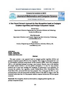
Test Results. Graphs (a), (b) and (c) in Figure 1 show the ratio of the number of correct pairs identified to the number of matchable pairs, in percent, for all the different particle concentrations and different proportions of unmatchable images considered. There is a graph for each of the three fluid flows considered, each graph showing together the performance of our neural network, that of the Grant and Pan network, and that of the nearest-neighbor algorithm, for comparison. The average success rates, calculated with all instances of a given flow type, for our neural network and that of Grant and Pan, differ by a negligible -0.3% for the Poiseuille flow, by 11.8% for the flow in a corner and by 28.6% for the vortex flow.
Graphs (b), (d) and (f) in Figure 1 show, for these same physical situations, the ratio in percent of the number of wrong pairs identified to the number of matchable pairs. They indicate that the proportion of false pairs produced by the three algorithms is consistent with the proportion of correct
16
pairs, and thus the former does not drastically lower the quality of the velocity field representation provided by the latter.
Figure 2 illustrates the difficulty of the matching problem when there are 200 particle images per picture, 40 of which are unmatchable. It shows a superposition of the two pictures, that is equivalent to a double exposure picture, for the fluid flow in a 900 corner. With this data, our neural network identified 156 of the 160 pairs correctly, producing the displacement field shown in Figure 3. Figure 4 shows the two different displacement fields produced by our neural network and that of Grant and Pan for an instance of the vortex flow problem.
5. CONCLUSION Our tests show that our neural-network can efficiently solve the correspondence problem of Particle-Tracking Velocimetry. Their results, presented in the graphs of Figure 1, indicate that both this neural network and the Grant and Pan neural network, out-perform by far the nearest-neighbor algorithm. They also indicate that our neural network performs significantly better than that of Grant and Pan for flows in which there are important changes in direction.
We recall that we lacked the details of the optimal weights initialization procedure for the Grant and Pan network. Because of this, we needed some reassurance that our conclusions would not be radically changed, with a different
17
network initialization than the one we used. As a crude test, we repeated the solution of the vortex flow problem of Figure 4, after initializing the weights of the Grant and Pan network with all of the correct particle image pairs. Surprisingly, its success rate actually went down to 54%, from 55% of correct pairs identified, thus leaving our network ahead with its identification of 78% of the correct pairs. Whatever the optimal initialization procedure may be for the Grant and Pan network, it remains that the latter network has to be taught about the fluid flow before being able to solve the correspondence problem. Our network, on the other hand, has the advantage of being completely self-starting and self-learning.
Another important difference and advantage of our neural network is the inherent parallelism of its operation. For all the instances of the problems considered above, a parallel realization of it would have produced the solution in 12 to 24 units of time. The Grant and Pan network, on the other hand, obtains its solution as a sequential process, that takes a number of steps directly proportional to the number of particle images in the first picture, i.e. 100 or 200 in the above examples.
Having demonstrated the potential of our neural network, we still have to do some work on determining the parameter values, the neighborhood function and the rate of decrease of the neighborhood radius, that would make it produce optimal results. Future work will also involve dealing with experimental data.
18
Finally, we remark that the performances of new algorithms often have to be compared to that of others. It is then very inefficient if, in order to do this, one has to implement the algorithms of others and try to optimize their parameters... It actually becomes very difficult when all the implementation details of the other algorithms are not available. A straightforward way to solve this problem is to have, accessible on the Internet, standard data sets that would be used for testing algorithms. With this in mind, we have made the data used in the present article available at the author's Internet page, that can be reached from the address http://www.rmc.ca
19
REFERENCES
Adrian RJ (1991) Particle-Imaging Techniques for Experimental Fluid Mechanics, Annual Review of Fluid Mechanics, 23, 261-304.
Carosone F, Cenedese A and Querzoli G (1995) Recognition of partially overlapped images using the kohonen neural network, Exp Fluids 19, 225-232.
Carpenter GA and Grossberg S (1987) ART2: self-organization of stable category recognition codes for analog input patterns. Applied Optics 26, 49194930.
Frieden BR and Zoltani CK (1989) Fast tracking algorithm for multiframe particle image velocimetry data. Applied Optics, 28, 652-655.
Grant I and Liu A (1989) Method for the efficient incoherent analysis of Particle Image Velocimetry images. Applied Optics 28, 1745-1748.
Grant I and Liu A (1990) Directional ambiguity resolution in Particle Image Velocimetry by pulse tagging. Exp Fluids 10, 71-76.
Grant I and Pan X (1995) An investigation of the performance of multi layer neural networks applied to the analysis of PIV images. Exp Fluids 19, 159-166.
20
Hassan YA and Philip OG (1997) A new artificial neural network tracking technique for particle image velocimetry. Exp Fluids 23, 145-154.
Hopfield JJ and Tank T (1985) Neural Computation in Optimization Problems. Biological Cybernetics 52, 141-152.
Knaak M Roghlübbers C and Orglmeister R (1997) A Hopfield Neural Network for Flow Field Computation Based on Particle Image Velocimetry/Particle Tracking Velocimetry Image Sequences, in the Proceedings of the 1997 International Conference on Neural Networks (ICNN '97) held at Houston Texas, published by IEEE, IEEE Catalog Number 97CH36109, 48-52.
Kohonen T (1982) A simple paradigm for the self-organized formation of structured feature maps. In Amari S and Arbib M ¨(Eds.), Competition and Cooperation in Neural Nets. Lecture notes in biomathematics, 45, SpringerVerlag.
Kohonen T (1984) Self-organization and associative memory. Berlin, SpringerVerlag.
Labonté G (1998) A SOM Neural Network That Reveals Continuous Displacement Fields. In the Proceedings of the 1998 International Joint Conference on Neural Networks at WCCI '98 (the World Congress on
21
Computational Intelligence), held at Anchorage Alaska, published by IEEE, IEEE ISBN 0-7803-4862-1.
Perkins RJ and Hunt JCR (1989) Particle tracking in turbulent flows. In Advances in Turbulence, 2, 286-291. Berlin, Springer-Verlag.
Uemura T, Yamamoto F and Ohmi K (1989) A high speed algorithm of image analysis for real time measurement of two-dimensional velocity distribution. In Flow Visualization, ed. Khalighi B, Braun M, Freitas C, FED-85, 129-134, New York, ASME.
Warsi ZUA (1992) Fluid Dynamics, Theoretical and Computational Approaches. Boca Raton, Florida: CRC Press, Inc.
22
100
100
80
80
60
60
40
40
20
20
0 100 90
80 70
60 200 180 160 140 120
0 100 90
80 70 60 200 180 160 140 120
(a)
(b)
100
100
80
80
60
60
40
40
20
20
0 100 90 80
70 60 200 180 160 140 120
0 100 90 80
70
(c)
(d)
100
100
80
80
60
60
40
40
20
20
0 100 90 80
70 60 200 180 160 140 120
(e)
60 200 180 160 140 120
0 100 90
80 70
60 200 180 160 140 120
(f)
Figure 1: The graphs (a), (c) and (e) show the ratios of the number of correct pairs identified to the number of matchable pairs, and (b), (d) and (f) that of false pairs, in percent. The percentage is shown along the vertical axis, the number of matchable pairs is along the horizontal axis. Two sets of curves are shown on
23
the same graph: those with the first 5 coordinates on the horizontal axis are for 100 particle images per picture, and those with the last 5 for 200. The solid curve corresponds to our neural network, the long-dashed curve to that of Grant and Pan, and the dotted curve to the nearest-neighbor algoritm. Graphs (a) and (b) are for the Poiseuillle flow, (c) and (d) for the flow in a 900 corner, (e) and (f) for the vortex flow.
Figure 2: Superposition of the two pictures of the particles, for the flow in the 900 corner formed by the left and bottom sides of the picture. The darker images belong to the first picture and the white ones to the second. Each picture has 200 images, 40 of which do not have a partner in the other picture.
24
Figure 3: Displacement field determined by our neural network from the data shown in Figure 2; 156 of the 160 image pairs are correctly identified.
(a)
(b)
25
Figure 4: In (a), displacement field determined by our neural network, with 78% of the pairs identified, and in (b) by the Grant and Pan network, with 55% of the pairs identified. The flow is a point vortex flow, with 200 particle images per picture, 40 of which are unmatchable.
26