21st International Conference on VLSI Design
A New Threshold Voltage Model for Omega Gate Cylindrical Nanowire Transistor Biswajit Ray Nano Scale Device Research Lab, CEDT, Indian Institute of Science Bangalore-560012
[email protected]
Santanu Mahapatra Nano Scale Device Research Lab, CEDT, Indian Institute of Science Bangalore-560012
[email protected] formulate simple compact models for these omega gate nanowire FETs for its successful implementation in future VLSI. Most of the previous works on the cylindrical nanowire structure are based on three dimensional numerical simulations [2, 4]. However, an analytical model for the threshold voltage and potential distribution was presented in [5] for fully surrounding gate nanowire transistor, which is the special case of more general omega gate MOSFET geometry. In this paper we propose an analytical model for calculating the potential Ψ(r,θ) at any point of the wire cross section of omega gate transistor based on the closed form solution of Poisson’s equation. Using the analytical expression of Ψ(r,θ) we have modeled the inversion charge and threshold voltage for the long channel undoped omega gate device. The models are then verified with the results obtained from professional three dimensional numerical device simulator [6].
Abstract In this work, for the first time, we present a physically based analytical threshold voltage model for omega gate silicon nanowire transistor. This model is developed for long channel cylindrical body structure. The potential distribution at each and every point of the of the wire is derived with a closed form solution of two dimensional Poisson’s equation, which is then used to model the threshold voltage. Proposed model can be treated as a generalized model, which is valid for both surround gate and semi-surround gate cylindrical transistors. The accuracy of proposed model is verified for different device geometry against the results obtained from three dimensional numerical device simulators and close agreement is observed.
1. Introduction To continue the CMOS (Complementary Metal Oxide Semiconductor) scaling trend for the next decade several non-classical MOSFET (Metal Oxide Semiconductor Field Effect Transistor) architecture have been proposed which offer better electrostatic integrity, higher transconductance and lower subthreshold swing than the traditional MOSFETs [1]. Double-gate Silicon on insulator (SOI) devices, multiple gate FinFETs and surrounding gate nanowire transistors are few examples of such attractive device structures. Although the surrounding gate devices offer the best immunity to Short Channel Effect (SCE) and Drain Induced Barrier Lowering (DIBL) [2], these structures requires complex processing steps that are difficult to make compatible with conventional CMOS fabrication processes. Considering the issues of mass production, semi-surrounded omega shaped gate structure has been proposed [3] to make a compromise between the device performance and manufacturability. Hence it is very important to
1063-9667/08 $25.00 © 2008 IEEE DOI 10.1109/VLSI.2008.52
Gate Oxide
Metal Gate X
Sillicon Nanowire O
α Q
P XX Buried Oxide
Si Wafer
Figure 1. Cross sectional view of the omega gate cylindrical Si nanowire transistor
447
Now the Eq. (1) can be divided into two following equations
2. Derivation of Potential model
ψ1
The cross section of a omega gate transistor for which we have developed our model is shown in Fig 1 The assumptions used for the derivation of the potential model are as follows: i) The channel is assumed to be undoped (intrinsic), as in these ultra thin body devices, SCE and DIBL are controlled by the device geometry rather than channel doping. Also the addition of dopants would lead to detrimental statistical fluctuations of threshold voltage. ii) The model is derived for long channel nMOS devices and the gradual channel approximation [7] has been used in solving the Poisson’s equation. iii) Effects of energy quantization in the inversion layer are not considered in the present work. With the above assumptions the 2D-Poisson’s equation along a vertical cut (X-XX) can be written in terms of polar coordinates as follows [5]: ∇ 2ψ (r , θ ) =
q
ε Si
ni
∇ 2ψ 1 (r ) = VT δ e VT
with boundary condition: ψ 1 ( R ) = ψ S and 2
∇ ψ 2 ( r , θ ) = VT δ e
ψ 1 (r ) = VT log
− 1)
(6) (7)
8B (1 − Br 2 ) 2 δ
(8)
where the constant B is evaluated from the boundary condition (5) and hence related to ΨS as below: ψS A 1 2 R 2 4 − VT + − + 1 1 1 , A = e (9) A δ R 2 R 2 It can be shown that for all practical values of ΨS the following relation holds good which makes the logarithmic term in Eq (8) real. 0 < BR 2 < 1 (10)
B=
(1) (2)
− qV
q 2 ni kT kT e , VT = , q being the kTε Si q electronic charge, ni the intrinsic carrier concentration , εSi the permittivity of silicon, V the electron quasiFermi potential, ΨS is the surface potential with g(θ) as a correction term which takes care of potential of the area which is not covered by the gate. It should be noted that the RHS of the Poisson’s equation contains only the mobile charge term (assumption (i)) and also valid for the gate voltage higher than flat band voltage (VFB), where the hole concentration could be neglected. Now for the surrounding gate nanowire transistor, due to symmetry, equation (1) reduces to onedimensional ordinary differential equation which can be solved analytically [5]. But in the case of omega gate FET, as the channel is not fully surrounded, we have to solve the two dimensional non linear partial differential equation to obtain potential profile Ψ(r,θ). To solve the equation (1) we split the total potential profile as follows:
where δ =
ψ (r , θ ) = ψ 1 (r ) + ψ 2 (r , θ )
(e
ψ2 VT
Equation (4) can be analytically solved as in the case of surrounding gate nanowire FET [5] with solution
ψ
with boundary condition : Ψ(R , θ) = ΨS + g(θ)
ψ1 VT
with boundary condition: ψ 2 ( R, θ ) = g (θ )
q (ψ −V ) e kT
= VT δ e VT
(4) (5)
Now, to solve the Eq. (6) we use the series expansion of the exponential term in braces and take first two terms only. This approximation is found to be an excellent one for points near the central region of the channel but deviates slightly at the points near boundary where the gate is not covered. With this approximation Eq (6) reduces to ψ1 2
∇ ψ 2 (r , θ ) = δ e VT ψ 2
(11)
Or ∂2
1 ∂ 1 ∂2 8B ψ2 + 2 ψ2 = ψ2 2 r ∂r r ∂θ (1 − Br 2 ) 2 ∂r (12) One needs to determine the exact form of boundary condition g(θ) in order to solve this non linear partial differential equation. From the simulation we perceive that g(θ) can be approximated by the following empirical expression πθ g (θ ) = C cos for −α ≤ θ ≤ α 2α = 0 otherwise. (13)
ψ2 + 2
(3)
448
0.7
0.62 Simulation
Surface Potential [V]
Potential (V)
0.6
Model
0.6 0.58 0.56 0
0.54 0.52
R=5nm,α=45 C=−.045
0.5 0.4 Model Simulation
0.3 0.2 0.1
R=10nm,α=450 C= −.07
0
0.5 −180 −120 −60 0 60 θ (Degree)
120 180
0
GS
Figure 2. Potential distribution at the boundary of the nanowire( (R, )) as a function of , plotted for two different radius values with the corresponding fitting parameter values mentioned in the figure
2
0.6 Model
0.58
Model
0.56
Simulation
simulation
R=10nm
α = 00
Potential [V]
Potential [V]
1.5 [V]
Figure 4. Surface potential variation as a function of Gate voltage. R=10nm. α = 45 0 , mid gap metal is used as gate and TOX = 2nm.
0.6
0.55
0.5 1 Gate Voltage V
α =300 0.5
0.54
R=15 nm 0.52
0
α=0 α=300
0.5 0.48 0.46
0
α =45 0.45 −10
−5
0 X [nm]
5
0
α=45
0.44 −15−12 −9 −6 −3 0 3 X [nm]
10
6
9 12 15
(b) R= 15nm
(a) R= 10nm
Figure 3. Potential distribution for different α along the vertical diameter (X-XX) (shown in the fig. 1) for two different radii. For both the cases VGS = 1V, mid gap metal is used as gate and TOX = 2nm. Hence we solve Ψ2 only for that region and as derived in the Appendix the solution for Ψ2 can be written as (for any practical values of α )
where C is a fitting parameter . With this approximation the potential profile at the boundary Ψ(R ,θ) is plotted along with simulation result in Fig. 2. We also observe from the simulation studies that the contribution from Ψ2 to the total potential distribution Ψ is significant only for the uncovered region of the body ( −α ≤ θ ≤ α ; that is the sector OPQ in Fig 1).
2
ψ 2 (r , θ ) = λ g (θ ) r 2k e −2 Br M (k + 1, 2k + 1, 4Br 2 ) (14) where M is the Kummer’s function [8] of first kind, λ is a constant determined from the normalizing
449
condition discussed in Appendix and k is a constant depending on α as
π k= 4α
QT = ε Si ∫ E.dS S 2π
(15)
= ε Si
Now, since it has been reported [4] that for the 75% gate coverage ( α = 45 0 ) the performance of omega gate nanowire transistor becomes very close to surrounding gate transistor, hence we present a simpler expression for potential distribution for the special case of α = 45 0 for which k=1 k = 1 . Now, for k = 1 the expression of ψ 2 simplifies to ψ 2 ( r ,θ ) = ψ 2 ( z = 2 Br 2 ,θ ) =
λ 2B
g (θ )(e z −
Hence the surface charge density is Q=
ε QT = Si 2πRL 2π
2π
∫ E.dθ
(19)
0
where L is the length of the channel and E is the electric field given by
(16) Hence the overall Potential model for the omega gate nanowire transistor ( for α = 45 0 ) reduces to
E=
dψ dr
(20) r=R
Now expression for Q can be analytically evaluated for any value of α , as shown at the bottom of the page (Eq. (21)).But a much simpler expression can be obtained for the special case of 75% gate coverage that is α = 45 0 which is written below:
8B λ sinh(z) + ) g(θ ) (ez − 1 2 2B z δ (1 − z) 2 2 where z = 2Br . (17)
ψ (r,θ ) = VT log
Using the general potential model the potential distribution has been plotted in Fig 3 along the vertical diameter (X-XX in Fig 1) for different α values. A closed agreement between model and numerical simulation (obtained from Sentaurus Device Simulator [6]) has been observed except at the oxide box boundary. This is because at the boundary some of the approximations used for explicit solution are not very accurate. But this minor deviation at the boundary will be smoothened out while we integrate this expression over θ for the calculation of total inversion charge and the threshold voltage.
Q=
2ε Si VT Z λCR2 sinh (Z ) + (Z eZ − cosh (Z ) + R (1 − .5Z ) 2π Z Z
where Z = 2BR 2
(22)
Now the variation of inversion charge with gate voltage is plotted in Fig 5 using Eq (21). We note that for a given gate voltage inversion charge decreases as we increase α which is expected because for higher α channel is less covered by gate. The definition of threshold voltage that is used for bulk MOSFET (gate voltage at which Ψs = 2φB; whereφB is the separation between extrinsic and intrinsic Fermi level) does not apply for undoped body devices. In this work, we define the threshold voltage for the omega gate nanowire transistor as the gate voltage for which the Ψs = ½EG (EG is the band gap for Si). With this definition, the threshold voltage of the device can be written as shown in the following Eq:
3. Inversion charge and threshold voltage Once the potential distribution at every point of the cross section of the cylindrical channel is known we can calculate the inversion charge density (Cm-2) by using Gauss law over the surface area of the channel. The total charge inside the cylindrical nanowire channel is given by (using Gauss law)
Q = ε Si
(18)
0
sinh( z ) ) z
2 C λα − 2 BR 2 4V T BR 1 − BR 2 + π 2 e
∫ E.R(dθ ) L
( 2 kR 2 k −1 − 4 BR 2 k +1 ) M ( k + 1 , 2 k + 1 , 4 BR 2 ) 2 k +1 2 k + 2 2 M ( k + 2 , 2 k + 2 , 4 BR ) + 4 BR 2k + 1
450
(21)
0.03
0
Threshold Voltage VTh (V)
Inversion Charge Q (C/m2)
α =0
0.025
0
α =30
0
α = 45
0.02
α =600 0.015 0.01 0.005 0
0
Simulation, α = 0 0
Model, α = 30
0.84
Simulation, α = 300
0.82
Model, α = 450 0
Simulation, α = 45
0.8 0.78 0.76 0.74 0.72
0
0.5 1 Gate Voltage V
GS
1.5 (V)
2
5
VTH = V FB +
EG Q + 2 C ox
ε ox (π − α ) πR log(1 + Tox / R )
15
Fig. 6. Threshold voltage variation for different gate coverage (or ) as a function of different nanowire radii values. Mid gap metal is used as gate and TOX = 2nm.
Although this expression is derived for 75% gate coverage, the error is found to be very small (less than 5%) if the same model is used for (± 10% extra) other gate coverage. However if we need the exact value we can use the general expression for Q in Eq. (23) for threshold voltage calculation. In Fig 6 the variation of threshold voltage has been plotted for various set of values of R & α by considering general expression for Q and verified with simulation results.
(23)
where VFB is the flat band voltage, Q is defined in the equation (21) and Cox can be calculated by the same procedure used as in the case of co-axial gate geometry [9] .The only modification we do here is that we assume the field in the uncovered region of the nanowire to be zero and neglect the fringing fields at the two ends of the omega gate (which are indeed good approximations as verified by simulation). With this modification the gate capacitance for omega gate structure can be given by C ox =
10
Radius [nm]
Fig. 5 Inversion charge (Cm-2) variation as a function of gate voltage using equation (7), for different . R=10nm.
4. Conclusion
(24)
where εox is the permittivity of oxide and Tox is the oxide thickness. Hence the final expression for threshold voltage for 75% gate coverage can be expressed as VTH
Model, α = 0
0.86
0
EG 2ε SiVT Z λCR2 sinh (Z ) Z = VFB + + + (Z e − cosh (Z ) + 1 COX R Z 2 2π Z (1 − Z ) 2
(25)
In this paper an explicit potential distribution model is derived for the cross sectional area of omega gate cylindrical nanowire transistor by solving the 2-D Poisson’s equation. Analytical expressions for the inversion charge and threshold voltage are also been presented. A simple compact model for potential distribution and threshold voltage has also been presented for the special case of 75% gate coverage (α = 450 ).The model is verified with 3D numerical simulation result and a good agreement has been found between the model we have introduced and the classical 3-D numerical simulation results.
5. Appendix To solve this partial differential equation (12) in the interval −α ≤ θ ≤ α we use variable separation technique and re-expressed Ψ2(r, θ) as
where the various terms are defined as in earlier Eqs.
451
ψ 2 (r , θ ) = φ1 (r )φ 2 (θ )
section is finite. Hence we let λ 2 = 0 . The other constant λ1 can be calculated from the boundary condition φ1 ( R) = 1 or
(26)
With this representation the partial differential Eq (12) can be separated into two ordinary differential eq as shown below: φ″ φ′ φ2″ 8Br 2 = − = ω 2 (27) r2 1 + r 1 − φ1 φ1 (1 − Br 2 ) 2 φ2
2
λ r 2 k e −2 Br M (k + 1, 2k + 1, 4 Br 2 ) So , the solution can be written as
ψ 2 (r, θ ) = λ r e
This work has been supported by Department of Science and Technology (DST), India.
(29)
7. References
Hence we let φ1 ( R) = 1 and solve to get
π
[1] J.-P. Colinge, “Multiple gate SOI MOSFETs,” Solid State Electron., vol. 48, no. 6, pp. 897-905, June 2004.
(30)
2α
[2] J.Wang, E. Polizzi, and M. Lundstrom, “A computational study of ballistic silicon nanowire transistors,” in IEDM Tech. Dig., Dec. 8–10, 2003, pp. 695-698.
To solve the radial part φ1 we approximate the (1 − Br 2 ) −2 term as (1 + 2 Br 2 ) as Br 2