Progress In Electromagnetics Research M, Vol. 12, 229–245, 2010
A NOVEL PHASE RETRIEVAL APPROACH FOR ELECTROMAGNETIC INVERSE SCATTERING PROBLEM WITH INTENSITY-ONLY DATA Y. Xiang, L. L. Li, and F. Li Institute of Electronics, Chinese Academy of Sciences Beijing, China Abstract—To measure the phase of signal with very high working frequency such as THz, and optics band is still a challenging problem. In this paper, based on the relationship between radiating current and measured intensity of electrical field a novel phase retrieval algorithm has been developed. As opposed to the existing approaches of phase retrieval where usually the Fourier coefficients of measured data will be firstly reconstructed, the proposed approach is to reconstruct the so-called radiating currents, with more physical meaning than the former. It has a much smaller number of freedoms of radiating current than that of measurements, which means that the obtained equations are over-determined. Thus one can efficiently model the intensity of measured electric field via the radiating part, and reconstruct it quickly and stably. The novelty is that this physical consideration 1) leads to efficiently avoiding false solutions due to the ill-posedness of phase retrieval problem, and 2) offers a good initial guess for inverse scattering based imaging algorithm. Importantly, a closed-form formulation of phase retrieve also has been derived when the intensity of incident wave is much stronger than one of the scattered wave, for example, for the weak scattering objects. Finally, several numerical experiments are provided to show the high performance of proposed algorithm. 1. INTRODUCTION Electromagnetic inverse scattering problem has been extensively studied for years for its theoretical significations and widely applications in medical imaging, industrial diagnostics, remote sensing, application geophysics, etc. The aim of EM inverse scattering is to Corresponding author: F. Li (
[email protected]).
230
Xiang, Li, and Li
retrieve the support and dielectric properties of unknown objects in a finite region by illuminating them with electromagnetic field and measuring the induced field outside the region. Both the intensity and phase information of the induced field are needed. However, the phase measurement generally presents more considerable practical difficulties and non-negligible hardware cost as the working frequency increases. Also the phase is very sensitive to the probe shaking and tends to be easily corrupted by noise in high frequency (especially beyond 10 GHz). Recently, one of the research interests in EM inverse scattering problem is on how to solve the problem without the phase information of the measured field [1–12]. Many results on the EM inverse scattering problems with onlyintensity information have been reported in [1–8]. Except for the methods based on linear approximations or a priori information of the support of the objects [6–8], there are two popular ways to deal with intensity-only data in the field of EM inverse scattering. One is to use the intensity-only data directly in the inverse procedure, called as one-step strategy [13, 14]. In this one-step strategy, the reconstruction error is easily to be measured whereas the nonlinearity of the problem is higher than that with full data case (FD, with the information of both phase and intensity), which causes the optimization procedure easily be trapped by local minimums and slow down the convergence [15]. An alternate is to reconstruct the phase of data from their amplitude first, and then run a standard FD inverse procedure [1–5]. Obviously, the accuracy and stability of phase retrieval will be the key issue to obtain successful reconstruction of probed obstacles. The present work mainly focuses on the phase retrieval where the incident field is known at any position and the intensity of the total field are measured by the receivers as carried out in many practical applications [10–12, 16]. It is along the line of our previous work [21] but gives more contents. Though many other excellent algorithms of phase retrieval have been developed, how to avoid the local solution by incorporating suitable prior information such as support and zero-point information of unknown signals is still a challenging problem [17]. For these exiting approaches, a commonly used approach is to reconstruct the coefficients in the Fourier domain with less physical meaning. As a matter of fact, due to the number of Fourier coefficients to be reconstructed, even the reduced-order Fourier transform, is much larger than one of independent data, the intrinsic ill-posedness cannot be efficiently overcame. To address this issue, the “originate” of measured data, i.e., the well-known radiating current source, is tracked based on the so-called electrical integral equation. As shown below, the freedom degree of radiating current
Progress In Electromagnetics Research M, Vol. 12, 2010
231
denoted by the number of efficient singular vectors of Green’s function usually is much lower than one of measured data. Consequently, the original underdetermined problem is turned into an over determined problem. Taking this point into account, a pleasing phase-retrieval algorithm is proposed, in particular, the radiating current firstly will be reconstructed by minimizing a cost function that relates the incident field, the intensity-only total field and the modeled scattered field, the coefficients of the series is retrieved iteratively, followed by computing the phase by simple relation between radiating current and the measured field. Our approach performs well for two reasons: 1) only the radiating part can affect and be reflected by the scattered field, 2) the number of the independent unknowns of the radiating part limited by the number of the significant singular values of the scatter operator, leading to a fast and stable convergence. Moreover, the radiating part can give an estimation of the objects’ support in multi-view case and can be used to reconstruct the non-radiating part of the equivalent currents as well as the objects dielectric properties directly in the inverse scattering step [18]. In Section 2, we first describe the relationship between the measured electric field and the equivalent radiating current, derive the corresponding cost function, and then discuss the method we use to minimizing the cost function and retrieve the phase of measured data. In Section 3, we test our phase-retrieval method with simulation and experiment data, and give some imaging results. In the final section, we conclude the paper and discuss the advantage of our method. 2. RECOVER PHASE INFORMATION FROM AMPLITUDE-ONLY MEASUREMENT 2.1. Image Principles of Inverse Scattering In this section some basic principles and notions involved in this paper have been summarized for the convenience of discussion. For simplicity, we just consider the two-dimensional scalar inverse scattering problem in homogeneous background, which also can be generalized into the three-dimensional full vectorial case along the same line. As shown in Fig. 1, the object(s) to be detected are assumed to be located in some region noted by the investigation domain. The unknown object is illuminated with EM wave and the amplitude of total field produced by the interaction between the object and incident wave is measured at some positions denoted as observation domain (outside the investigation domain). This procedure can be described by two integral
232
Xiang, Li, and Li
Figure 1. The measurement setup. equations called data equation and state equation respectively [1]: Escatt (ρr ) = Etot (ρr ) − Einc (ρr ) Z ¡ ¢ ¡ ¢ ¡ ¢ 2 = kb Gd ρr , ρ0 · Etot ρ0 χ ρ0 dρ0 , ρr ∈ Dobs , ρ0 ∈ Dinv Dinv
Z
(1)
¡ ¢ ¡ ¢ 0 ¡ ¢ Gs ρ, ρ0 ·Etot ρ0 χ ρ0 dρ , ρ, ρ0 ∈ Dinv (2)
Einc (ρ) = Etot (ρ)−kb2 Dinv
where Einc , Escatt , Etot are the incident field, scattered field and total field, respectively, kb is the background wave number, Dinv denotes the investigation domain and Dobs denotes the observation domain, Gd is the Green’s function mapping Dinv to Dobs , and Gs is the Green’s function mapping Dinv to Dinv itself. The function χ(·) = ε(·)/εb (·) − 1 + iσ(·)/ωεb (·) demonstrates the contrast distribution of the unknown objects which is expected to be determined in the inverse scattering problems, where ε is the dielectric permittivity of the objects, εb is the one of the background, σ is the conductivity of the objects. Since the unknown objects are all located inside Dinv , χ(·) becomes zero outside that region. The two dimensional scalar Green’s (1) function is given by G(ρ, ρ0 ) = 4i H0 (kb |ρ − ρ0 |), expressed in terms (1)
of the Hankel function H0 of order zero and of the first kind. Indeed, the product of the contrast function and the total field in Dinv is the so-called contrast source defined by w(·) = χ(·)Etot (·), which implies the equivalent current density on the supports of the objects. Above two equations are the standpoints of electromagnetic inverse scattering problem described in the frequency domain.
Progress In Electromagnetics Research M, Vol. 12, 2010
233
2.2. Establishment of the Cost Function In this subsection, we will investigate the relationship between amplitude of total measured electric field and the radiating current. If we only measure the amplitude information, Equation (1) can be modified as: ¯ ¯ ¯ ¯ Z ¯ ¡ ¢ ¡ 0¢ 0¯ 0 2 ¯ |Etot (ρr )| = ¯Einc (ρr ) + kb Gd ρr , ρ · w ρ dρ ¯¯ , ρr ∈ Dobs , ¯ ¯ Dinv
It is noted that the scattering operator
R
ρ0 ∈ Dinv (3) dρ0 Gd (ρr , ρ0 ) ◦ is of narrow
Dinv
bandwidth [19], which means that if we perform the singular value decomposition (SVD): Z Z X ¡ ¢ ¡ ¢ dρ0 Gd ρr , ρ0 ◦ = U` (ρr ) γ` dρ0 V`∗ ρ0 ◦ (4) `
Dinv
Dinv
where (·)∗ stands for the complex conjugate, {U` (ρr ), ρr ∈ Dobs } and {V` (ρ0 ), ρ0 ∈ Dinv } are the normalized orthogonal function series in R Dobs and Dinv respectively. Introducing P` = dρ0 V`∗ (ρ0 )w(ρ0 ), one Dinv has
Escatt (ρr ) =
X `
{σ` P` } U` (ρr )
(5)
This equation implies that only the part of w(ρ0 ) corresponding to the first few singular values can be contributed obviously to the scattered field. It is called as radiating current while the rest of w(ρ0 ) is called as the nonradiating current. After determining the radiating current one can derive the full data of Escatt via Equation (1). Analytical form of the SVD of the scattering operator can be derived for special case [19]. However, for different measurement setups and background, it is need to consider the SVD within the framework of a discrete form. By meshing Dinv into N equal sub-squares, in each of which the field, contrast and contrast source function are approximated to be constant, and the discrete version of Equation (3) is ¯ ¯ ¯ ¯ ¯ ¯ ¯ ¯ ¯ ¯ ¯ ¯ ¯[Etot ](r) ¯ = ¯[Einc ](r) + [Escatt ](r) ¯ = ¯[Einc ](r) + [[Gd ] [w]](r) ¯ , r = 1, 2, . . . , R
(6)
where [·] stands for the discrete form of a continues function and R is the number of receiver. The singular value decomposition (SVD) of [Gd ] is given by [Gd ] = [U ] [Σ O] [V ]∗
234
Xiang, Li, and Li
then [Escatt ] = [Gd ] [w] = [U ] [Σ O] [V ]∗ [w] = [U ] [Σ O] [P ] · R ¸ £ ¤ P = [U ] [Σ O] = [U ] [Σ] P R N R P
(7)
where [P ] = [V ]H [w], and [P R ], [P N R ] imply the radiating and nonradiating part, respectively, [Σ] = diag{γ 1 , γ 1 , . . . , γ R }, γ 1 ≥ γ 2 ≥ . . . ≥ γ j > 0, and γ j+1 = . . . = γ R = 0, [O] is a zero matrix. The series {γi , r = 1, 2, . . . , R} are the singular values of [Gd ] and decline rapidly to zero so that a truncation of them is usually made, refer to Section 3. Now Equation (7) is changed to R P1 σ1 . ... .. [Escatt ] ≈ [u1 | u2 | · · · | uT r ] σT r PTRr £ ¤£ ¤£ ¤ = U T r ΣT r P T r (8) Then
£ ¤£ ¤£ ¤ [Etot ] = [Einc ] + [Escatt ] ≈ [Einc ] + U T r ΣT r P T r
(9)
where Tr is the truncation index, [U T r ] is consisted with first Tr columns of [U ], [P T r ] is consisted with first Tr rows of [P ], and [ΣT r ] = diag{γ 1 , . . . , γ T r }. 2.2.1. Closed-form Solution to Phase Retrieve If |[Escatt ](r) | ¿ |[Einc ](r) |, r = 1, . . . , R, which usually happens when the objects of interest are weak scatterers, from (3) and (5) one has ¯ ¯2 ¯ ¯2 ¯2 ³ ´ ¯ ¯ ¯ ¯ ¯ ¯ ¯ ∗ ¯[Etot ](r) ¯ − ¯[Einc ](r) ¯ = 2Re [Einc ](r) [Escatt ](r) + ¯[Escatt ](r) ¯ ³ ´ ³ ££ ¤£ ¤£ ¤¤ ´ ≈ 2Re [Einc ]∗(r) [Escatt ](r) = 2Re [Einc ]∗(r) U T r ΣT r P T r (r) There is a linear relationship between |[Etot ]|2 − |[Einc ]|2 and the unknown [PT r ]. Consequently, define ¯ ¯2 ¯ ¯2 ¯ ¯ ¯ ¯ y = [yr ] , yr = ¯[Etot ](r) ¯ − ¯[Einc ](r) ¯ £ ¤ H = [hrt ] , hrt = γt [Einc ]∗(r) · U T r (r,t) , r = 1, . . . , R, t = 1, . . . , T r the P T r can be given explicitly by ¤ ¸ · £ Re £P T r ¤ = [Re [H] , −Im [H]]† y Im P T r
(10)
Progress In Electromagnetics Research M, Vol. 12, 2010
235
where [Re [H], −Im [H] ]† = ( [Re [H], −Im [H] ]T [ Re [H], −Im [H] ] )−1 [Re[H], −Im[H]]T . Once the radiating current P T r has been derived via Equation (10), the full data (amplitude plus phase) of scattering field can be readily obtained via Equation (5). 2.2.2. Iterative Solution to Phase Retrieve If |[Escatt ](r) | ∼ |[Einc ](r) |, r = 1, . . . , R, to obtain [P T r ] a iterative approach has to be exploited to solve a nonlinear optimization problem, in particular, [P T r ] can be reconstructed by searching the minimum of the cost function given by the square norm of the square error of measured and estimated intensity of the total field, which is defined as R ¯¯ ¯2 ¯ ¯2 ¯¯2 ¯¯££ T r ¤ £ T r ¤ £ T r ¤¤ ¡£ T r ¤¢ X ¯ ¯ ¯ ¯ Φ P = Σ P + [Einc ](r) ¯ − ¯[Etot ](r) ¯ ¯¯ ¯¯ U (r) r=1
The cost function is derived for the single-transmitter case in which the objects of interest are illustrated by electromagnetic wave from only one direction. For the multi-transmitter case, denote by S be the number of illustrating directions, [Einc ], [Escatt ], [Etot ] become matrix form, and the cost function can be written as ¡£ ¤¢ Φ PTr R X S ¯¯ ¯2 ¯ ¯2 ¯¯2 X ¯¯££ T r ¤ £ T r ¤ £ T r ¤¤ ¯ ¯ ¯ ¯ = Σ P + [Einc ](r,s) ¯ − ¯[Etot ](r,s) ¯ ¯¯ (11) ¯¯ U (r,s) r=1 s=1
The radiating current is given by searching the global minimum of the cost function, while its local minimum can be avoided by increasing the ratio of number of freedom of the measured data and that of the unknowns [17]. The radiating current, when expressed in the domain of [V ]∗ , has only a very few non-zero elements, i.e., [P T r ], which ensures a sufficient large ratio when the freedom of the measured data is fixed. In the next subsection, minimizing the cost function (11) via the PolakRibi`ere conjugate gradient approach is briefly outlined. 2.2.3. Minimizing the Cost Function by Polak-Ribi`ere Conjugate Gradient Method The Polak-Ribi`ere conjugate gradient method is exploited to minimize the cost function (11), where a key issue is to calculate the conjugate gradient of the cost function given as: ¡£ ¤¢ ∆ ∂Φ ∇Φ P T r = ∂ [P T r ]H £ ¤£ ¤H ¡ ¡ £ ¤£ ¤£ ¤¢¢ =2 ΣT r U T r ∆. ∗ [Einc ]+ U T r ΣT r P T r (12)
236
Xiang, Li, and Li
where ∆ = [∆r,s ] , ¯££ ¯2 ¯ ¯2 ¤£ ¤£ ¤¤ ¯ ¯ ¯ ¯ ∆r,s = ¯ U T r ΣT r P T r (r,s) + [Einc ](r,s) ¯ − ¯[Etot ](r,s) ¯
(13)
and the operator .∗ is defined as [A].∗[B] = [ar,s ].∗[br,s ] = [ar,s br,s ], the matrix [A] and [B] are of the same size. Let [GT r ] = −[∇Φ], and [DT r ] be the search direction. [GT r ] and [DT r ] are matrix of size R × T r. The minimizing procedure is summarized as: Initializing: £ ¤(0) n = 0, random choose P T r and set ³£ ¤(0) ´ £ T r ¤(0) £ T r ¤(0) = −∇Φ P T r = G D
(14)
WHEN no satisfied condition is obtained, DO £ ¤(n+1) £ T r ¤(n) £ ¤(n) STEP I: Computing P T r = P + α(n+1) DT r , and ³£ ¤(n) £ ¤(n) ´ α(n) = argα min Φ P T r + α V Tr (15) STEP II. Calculating £ T r ¤(n+1) £ T r ¤(n+1) £ ¤(n) D = G + β (n+1) DT r with ³£ ¤(n+1) ´ £ T r ¤(n+1) G = −∇Φ P T r and D E (n+1) (n) (n+1) −[GT r ] ,[GT r ] [GT r ] (n+1) D E β = [GT r ](n) ,[GT r ](n) PP ∗ where h[·] , [◦]i := [·](r,s) [◦](r,s) r s ¡£ ¤¢ STEP III. Checking if Φ P T r is lower than a given threshold. If not, goto STEP I; else computing the radiating part of [w] is given by · ¸ £ T r¤ PTr w = [V ] (16) 0
3. SIMULATION AND EXPERIMENT VALIDATION In this section, several numerical simulations and experiment studies have been carried out to test the performance of the proposed
Progress In Electromagnetics Research M, Vol. 12, 2010
237
algorithm. The experiment data is provided as a free resource for inverse scattering test by the Institute Fresnel in Marseille in France [16]. The setup of the measurement is shown by the Fig. 1, where the objects are located in a 0.15 × 0.15 m2 squares in free space, and the transmitter illuminate from eight directions on a circle with 1.67 m in radius, rounding this square. The incident angle θs changes from 0◦ ∼ 360◦ , by 45◦ per illumination. The receiver measures the electric field on the same circle. The receiving angle θr changes from 60◦ ∼ 300◦ , by 1◦ per sample. The working frequency for our all studies is set to be 2 GHz. Firstly, we carried out the numerical simulation for probed objects shown in Fig. 2(a), where the transmitter is modeled by an electric dipole. As mentioned above, the singular values of the Green’s matrix [Gd ] decrease rapidly as shown in Fig. 3, which means that the freedom of radiating current is much low, and with very small number of singular vector the radiating current can be represented with enough
(a)
(b)
(c)
Figure 2. Test objects: The relative permittivity of the white cylinder is 3.0, and that of the gray cylinder is 1.45.
Figure 3. The singular values of Green’s matrix.
238
Xiang, Li, and Li
accuracy. To address this issue, introduce the truncation error and reconstruction error of the scattered electric field density on measuring circle is defined as: k[Escatt ]tr − [Escatt ]ac k2 err tr = (17) k[Escatt ]ac k2 err rec =
k[Escatt ]rec − [Escatt ]ac k2 k[Escatt ]ac k2
(18)
where [Escatt ]tr is the approximate scattered field density given by (8), [Escatt ]rec is the reconstructed one given by the proposed method and [Escatt ]ac is the actual one, the truncation and reconstruction errors (noise free) for different choices of the truncation threshold T r are listed in Tab. 1. It shows that a larger T r leads to more accurate reconstruction. However, the convergence of the iteration process will be slowed down respectively, and the accuracy of the further reconstruction of object function will not be obviously improved. Here, the smallest T r such that γ T r /γ 1 < 1% is prefer. In noisy case, the present method can still give a very good reconstruction of the scattered field, which is shown in Fig. 4. Table 1. Reconstruction error with different truncation threshold. Tr 8 10 16 20
err tr 0.0608% 0.0014% 1.5098e-008% 3.9306e-013%
err rec 0.2011% 0.0230% 2.2959e-006% 7.5738e-008%
(a) (b) Figure 4. Reconstruction results with zero mean Gaussian noise, (a) phase of the scattered field, (b) amplitude of the scattered field.
Progress In Electromagnetics Research M, Vol. 12, 2010
(a)
239
(b)
(c)
(d)
(e)
Figure 5. The reconstruction for probed objects shown in Fig. 2(a): (a) Phase of the scattered field (θs = 0◦ ), (b) amplitude of the scattered field (θs = 0◦ ), (c) contrast map of the objects estimated by radiating equivalent current, (d) contrast map of the objects estimated by all equivalent current, (e) relative permittivity on the line y = 0.
240
Xiang, Li, and Li
(a)
(b)
(c)
(d)
(e)
Figure 6. The reconstruction for probed objects shown in Fig. 2(b): (a) phase of the scattered field (θs = 0◦ ), (b) amplitude of the scattered field (θs = 0◦ ), (c) contrast map of the objects estimated by radiating equivalent current, (d) contrast map of the objects estimated by all equivalent current, (e) relative permittivity on the line y = 0.
Progress In Electromagnetics Research M, Vol. 12, 2010
(a)
(b)
(c)
(d)
241
(e)
Figure 7. The reconstruction for the objects shown in Fig. 2(c): (a) phase of the scattered field (θs = 0◦ ), (b) amplitude of the scattered field (θs = 0◦ ), (c) contrast map of the objects estimated by radiating equivalent current, (d) contrast map of the objects estimated by all equivalent current, (e) relative permittivity on the line y = 0.
242
Xiang, Li, and Li
Secondly, based on the experimental data from Frenel Lab three test objects shown in Fig. 2 are used to test the proposed algorithm. The experiment data given by [20] include both real and imaginary part of the total and incident electric field density. We only utilize the amplitude information of the total field for reconstruction. Though the information of incident wave is not provided, it can be modeled with enough accuracy if the parameters of used antenna are known. For this case, the transmitters/receivers are modeled by an electric dipole. Afterwards, the scattered or total field is reconstructed by the proposed algorithm. The results are shown in Figs. 5 ∼ 7(a), 7(b), respectively for different test objects, As the by-product, the reconstructed radiating part of the equivalent current density to perform a coarse estimation of the dielectric properties of test objects also are shown in Figs. 5 ∼ 7(c). The estimations give good approximated contrast map of the test objects. Moreover, we also use the estimation as initial guess for inverse scattering reconstruction [18], shown in Figs. 5 ∼ 7(d), 7(e), respectively. 4. CONCLUSION In this paper, we have proposed a highly efficient algorithm to retrieve the phase information from the intensity-only measurement for the electromagnetic inverse scattering imaging, which can be used for the imaging application where phase measurement is difficult or highly expensive such as optics and THz imaging. The key point of the algorithm is to estimate the radiating part of the equivalent current from the amplitude-only data. Importantly, a closed-form formulation of phase retrieve, i.e., Equations (10) and (5), also has been derived when the intensity of incident wave is much stronger than one of the scattered wave, for example, for the weak scattering objects. In addition, the reconstructed equivalent radiating current is a byproduct of our algorithm. Furthermore, it can be used to give a coarse contrast map of test objects, which is helpful in fast imaging. Indeed, it also gives a good initial guess in further inverse scattering reconstruction. ACKNOWLEDGMENT This work is supported by National Natural Science Foundation of China under Grant No. 60701010 and No. 40774093 and National 863 plans projects 2008AA12Z104.
Progress In Electromagnetics Research M, Vol. 12, 2010
243
APPENDIX A. In this appendix, how to solve Equation (15) is summarized. Firstly, Equation (15) can be rewritten as ³£ ¤(n) £ ¤(n) ´ Φ PTr + α DT r R X S ¯ ¯2 X ¯ 2 ¯ = ¯α [A](r,s) +α [B](r,s) +[C](r,s) ¯ = aα4 +bα3 +cα2 +dα + e r=1 s=1
where a =
XX¯ ¯ ¯A(r,s) ¯2 r
b = 2Re
s
XX r
[A]∗(r,s) [B](r,s)
s
XX¯ ¯ ¯B(r,s) ¯2 + 2Re hA, Ci c = r
s
d = 2Re hB, Ci XX¯ ¯ ¯C(r,s) ¯2 . e = r
A(r,s)
B(r,s)
C(r,s)
s
¯h ¯2 ¯ £ T r ¤ £ T r ¤ £ T r ¤(n) i ¯ ¯ ¯ = ¯ U Σ D (A1) (r,s) ¯ ¶ µ h£ ¤£ ¤£ ¤ i T r ΣT r P T r (n) U [E ] + inc (i,j) (r,s) = 2Re h£ (A2) ¤ £ T r ¤ £ T r ¤(n) i∗ T r Σ D × U (r,s) i ¯ h£ ¯ 2 ¤ £ ¤ £ ¤ ¯ U T r ΣT r P T r (n) ¯ ¯ ¯2 ¯ ¯ ¯ ¯ (n) (r,s) ¯ − ¯[Etot ](r,s) ¯ = ∆r,s (A3) = ¯ ¯ + [Einc ] ¯ (r,s)
Correspondingly, the updating step size α(n+1) is the minimum real positive root of the equation by ³ ³£ ¤(n) £ ¤(n) ´´ + α V Tr ∂ Φ PTr = 4aα3 + 3bα2 + 2cα + d = 0 (A4) ∂α REFERENCES 1. Crocco, L., M. D’Urso, and T. Isernia, “Inverse scattering from phaseless measurements of the total field on a closed curve,” J. Opt. Soc. Amer., Vol. 21, No. 4, 622–630, Apr. 2004.
244
Xiang, Li, and Li
2. Bucci, O. M., L. Crocco, M. D’Urso, and T. Isernia,, “Inverse scattering from phaseless measurements of the total field on open lines,” J. Opt. Soc. Amer., Vol. 23, No. 10, 2566–2577, Oct. 2006. 3. Catapano, I., L. Crocco, M. Urso, and T. Isernia, “Advances in microwave tomography phaseless measurements and layered backgrounds,” Proc. 2nd Int. Workshop on Advanced GPR, 183– 188, Delft, The Netherlands, May 2003. 4. Caorsi, S., A. Massa, M. Pastorino, and A. Randazzo, “Electromagnetic detection of dielectric scatterers using phaseless synthetic and real data and the memetic algorithm,” IEEE Trans. Geosci. Remote Sensing, Vol. 41, No. 12, 2745–2753, Dec. 2003. 5. Franceschini, G., M. Donelli, R. Azaro, and A. Massa, “Inversion of phaseless total field data using a two-step strategy based on the iterative multiscaling approach,” IEEE Trans. Geosci. Remote Sensing, Vol. 44, No. 12, 3527–3539, Dec. 2006. 6. Maleki, M. H., A. J. Devaney, and A. Schatzberg, “Tomographic reconstruction from optical scattered intensities,” J. Opt. Soc. Am. A, Vol. 10, 1356–1363, 1992. 7. Maleki, M. H. and A. J. Devaney, “Phase retrieval and intensity-only reconstruction algorithms from optical diffraction tomography,” J. Opt. Soc. Am. A, Vol. 10, 1086–1092, 1993. 8. Takenaka, T., D. J. N. Wall, H. Harada, and M. Tanaka, “Reconstruction algorithm of the refractive index of a cylindrical object from the intensity measurements of the total field,” Microwave Opt. Technol. Lett., Vol. 10, 182–188, 1997. 9. Devaney, A. J., “Diffraction tomographic reconstruction from intensity data,” IEEE Trans. Imaging Process, Vol. 1, 221–228, 1992. 10. Maleki, M. H., A. J. Devaney, and A. Schatzberg, “Phase retrieval and intensity-only reconstruction algorithms from optical diffraction tomography,” J. Opt. Soc. Am. A, Vol. 10, 1086–1092, 1993. 11. Gbur, G. and E. Wolf, “Hybrid diffraction tomography without phase information,” J. Opt. Soc. Am. A, Vol. 19, 2149–2202, 2002. 12. Las-Heras, F. and T. Sarkar, “A direct optimization approach for source reconstruction and NF-FF transformation using amplitudeonly data,” IEEE Trans. Antennas. Propag., Vol. 50, No. 4, 500– 510, Apr. 2002. 13. Takenaka, T., D. J. N. Wall, H. Harada, and M. Tanaka, “Reconstruction algorithm of the refractive index of a cylindrical object from the intensity measurements of the total field,”
Progress In Electromagnetics Research M, Vol. 12, 2010
14.
15. 16. 17. 18.
19.
20.
21.
245
Microwave Opt. Technol. Lett., Vol. 14, 182–188, 1997. Caorsi, S., A. Massa, M. Pastorino, and A. Randazzo, “Electromagnetic detection of dielectric scatterers using phaseless synthetic and real data and the memetic algorithm,” IEEE Trans. Geosci. Remote Sens., Vol. 41, 2745–2752, 2003. Li, L. L., H. Zheng, and F. Li, “Two-dimensional contrast source inversion method with phaseless data: TM case,” IEEE Trans. Geosci. Remote Sens., Vol. 47, No. 6, 1719–1736, 2008. Hislop, G., G. C. James, and A. Hellicar, “Phase retrieval of scattered fields,” IEEE Trans. Antennas Propag., Vol. 55, 2332– 2341, 2007. Isernia, T., G. Leone, R. Pierri, and F. Soldovieri, “Role of the support and zero locations in phase retrieval by a quadratic approach,” J. Opt. Soc. Am. A, Vol. 16, 1845–1856, 1999. Caorsi, S. and G. L. Gragnani, “Inverse-scattering method for dielectric objects based on the reconstruction of the nonmeasurable equivalent current density,” Radio Science, Vol. 34, No. 1, 1–8, 1999. Chiappe, M. and G. L. Gragnani, “An analytical approach to the reconstruction of the radiating current in inverse electromagnetic scattering,” Microwave Opt. Technol. Lett., Vol. 49, No. 2, 354– 360, 2007. Geffrin, J., P. Sabouroux, and C. Eyraud “Free space experimental scattering database continuation: Experimental set-up and measurement precision,” Inverse Problems, Vol. 21, S117–S130, 2005 Xiang, Y., L. L. Li, and F. Li, “Inversion of phaseless total data by reconstruction the equivalent radiating current,” 2008 AsiaPacific Microwave Conference, (APMC 2008), 2008.