and neural network approach to estimate the impact of groundwater ... controlling
factors and the outputs from the numerical model simulations, providing an. 11.
1
The definitive version of this article was published by Elsevier as:
2
Parkin, G, Birkinshaw, S.J, Younger, P.L, Rao, Z. and Kirk, S. A numerical modelling
3
and neural network approach to estimate the impact of groundwater abstractions on river
4
flows. Journal of Hydrology 2007, 339(1-2), 15-28. doi:10.1016/j.jhydrol.2007.01.041
5
A NUMERICAL MODELLING AND NEURAL NETWORK
6 7
APPROACH TO ESTIMATE THE IMPACT OF GROUNDWATER
8
ABSTRACTIONS ON RIVER FLOWS
9 G Parkin1 , S J Birkinshaw1 , P L Younger2 , Z Rao3, S Kirk4
10
11
12 13
1
School of Civil Engineering and Geosciences, Newcastle University 2
Institute for Environment and Sustainability, Newcastle University 3
14 15
4
Halcrow Ltd
Environment Agency of England and Wales
16
Abstract
17
Evaluation of the impacts of groundwater abstractions on surface water systems is
18
a necessary task in integrated water resources management. A range of hydrological,
19
hydrogeological, and geomorphological factors influence the complex processes of
20
interaction between groundwater and rivers. This paper presents an approach which uses 1
1
numerical modeling of generic river-aquifer systems to represent the interaction
2
processes, and neural networks to capture the impacts of the different controlling factors.
3
The generic models describe hydrogeological settings representing most river-aquifer
4
systems in England and Wales: high diffusivity (e.g. Chalk) and low diffusivity (e.g.
5
Triassic Sandstone) aquifers with flow to rivers mediated by alluvial gravels; the same
6
aquifers where they are in direct connection with the river; and shallow alluvial aquifers
7
which are disconnected from regional aquifers. Numerical model simulations using the
8
SHETRAN integrated catchment modeling system provided outputs including time-series
9
and spatial variations in river flow depletion, and spatially distributed groundwater levels.
10
Artificial neural network models were trained using input parameters describing the
11
controlling factors and the outputs from the numerical model simulations, providing an
12
efficient tool for representing the impacts of groundwater abstractions across a wide
13
range of conditions. There are very few field data sets of accurately quantified river flow
14
depletion as a result of groundwater abstraction under controlled conditions. One such
15
data set from an experimental study carried out in 1967 on the Winterbourne stream in
16
the Lambourne catchment over a Chalk aquifer was used successfully to test the
17
modeling tool. This modeling approach provides a general methodology for rapid
18
simulations of complex hydrogeological systems which preserves the physical
19
consistency between multiple and diverse model outputs.
20 21
Keywords: groundwater, abstraction, river-aquifer interaction, neural networks,
22
numerical modeling
2
INTRODUCTION
1 2
It is recognized that surface and groundwater systems must be managed in an
3
integrated way to provide water supplies and to control water levels and flows while
4
addressing concerns over the conservation of the natural environment (e.g. Winter et al.,
5
1998). This has been recognized particularly in the EU Water Framework Directive,
6
which has increased awareness of the need for integrated catchment management.
7
One of the ways in which the environment can be degraded is through over-
8
abstraction of groundwater causing a reduction of baseflow to rivers. The direction and
9
rate of flow between an aquifer and a river depends on the hydraulic gradient and degree
10
of hydraulic connection. These are affected by factors including geology, contributing
11
catchment area, recharge rates, geomorphology of the channel and the surrounding land,
12
river stage, and river bed sediments. Fine sediments can cause significant resistance to the
13
flow of water between the river and aquifer (Younger et al., 1993), and in disconnected
14
rivers this can cause the aquifer material between the river-bed and the water table to
15
become unsaturated (Rushton, 2003).
16
The impacts of groundwater abstractions on the environment can be assessed
17
using a hierarchy of modeling tools, ranging from simple water balance calculations
18
through to regional numerical groundwater models, depending on the complexity and
19
importance of the site. The key features that need to be assessed in these models are the
20
depletions in river flows due to reduced baseflow contributions (or, in extreme cases,
21
reversals of groundwater flow direction leading to losing river reaches), when and where
22
these changes in baseflow occur, and the changes in groundwater levels near to river
23
channels. 3
1
Analytical models can provide simplified representations of the processes of
2
river-aquifer interactions, support of decision-making on siting or operation of abstraction
3
wells near rivers. Models have been presented addressing different configurations of
4
river-aquifer systems, including those of Theis (1941) for pumping from a fully-
5
penetrating well in an isotropic, homogeneous semi-infinite confined aquifer in full
6
hydraulic connection with a straight fully-penetrating stream, Hantush (1965) for the
7
same configuration but including a river bed layer with different (lower) permeability,
8
Hunt (1999, following earlier work by Stang, 1980) for a partially-penetrating river with
9
a semi-permeable bed, and Butler et al. (2001) for a heterogeneous aquifer.
10
Some of the limitations of these methods can be overcome by using numerical
11
modelling techniques (Dillon, 1983; Winter, 1984; Vasiliev, 1987; Younger, 1987, 1990;
12
Winter, 1995; Winter et al., 1998), although these are generally more time-consuming
13
and costly. A numerical model of river aquifer interactions usually involves separate
14
numerical solution of equations for surface water routing and groundwater flow, with
15
coupling between the two models often based on a simple Darcy calculation (Winter,
16
1995). This approach is followed in river-aquifer interaction add-on modules developed
17
for the MODFLOW groundwater model (McDonald and Harbaugh, 1988; Harbaugh and
18
McDonald, 1996), including the original RIVER module, the STREAM module (Prudic,
19
1989), and the BRANCH module which was combined with MODFLOW to create the
20
MODBRANCH model (Swain, 1994). Each of these has a different representation of
21
surface water routing, but uses essentially the same approach for calculating exchange
22
flows based on a conductance term. It has been argued that this term does not have a clear
23
physical meaning due to the common existence of three-dimensional flows and non-linear 4
1
responses near to rivers (McDonald and Harbaugh, 1988). Recent examples of using
2
MODFLOW for applications involving river aquifer interactions include Modica et al.
3
(1997), Chen et al. (1997), Carey and Chanda (1998) and Wroblicky et al. (1998).
4
Approximations to three-dimensional surface-groundwater coupling are included in some
5
models, e.g., SHETRAN (Ewen et al., 2000) and ICMM (van Wonderen and Wyness,
6
1995).
7
Comparisons between some analytical and numerical models and assessments of
8
the effects of the simplifications in the analytical models are given by Spalding and
9
Khaleel (1991), Sophocleous et al. (1995) and Conrad and Beljin (1996). In these studies,
10
significant errors in the analytical solutions were related to fully penetrating rivers, and
11
lack of representation of river sediments and aquifer storage beyond the stream. Some of
12
the limitations of analytical models reported in these comparative studies have since been
13
overcome (e.g. Butler et al., 2001). However, some processes leading to non-linearities in
14
behaviour cannot easily be modeled using analytical methods, for example the behaviour
15
of disconnected rivers, multiple aquifers connected to rivers, changes in transmissivity
16
within the cone of depression, and seasonality of recharge inputs which will affect the
17
timing of variations in groundwater levels and baseflows. New methods that could
18
address these issues without the cost and effort of building a numerical model for each
19
assessment would therefore provide a beneficial approach to supporting abstraction
20
borehole siting and operation.
21
Di Matteo and Dragoni (2005) derived an empirical relationship linking a set of
22
parameters controlling steady-state stream flow depletion in a highly inter-connected
23
river-aquifer system as a result of abstraction from a partially penetrating well, by 5
1
running a set of numerical model simulations. They noted the limits of validity of the
2
relationship, and that the stream flow depletion was insensitive to some parameters in
3
certain areas of the response surface. Artificial neural networks (ANN’s) are one
4
promising method which can be used to represent more generalized relationships. An
5
ANN is a set of highly interconnected mathematical processing elements which are
6
capable of representing non-linear multivariate mapping functions between input and
7
output data sets. The forms of the mapping functions are determined through ‘training’
8
the ANN using sets of input and output data. Although most applications of ANN’s in
9
hydrology and water resources are data-driven, some previous studies have been carried
10
out using a similar hybrid approach with numerical models (Rao and Jamieson, 1997;
11
Rao and O’Connell, 1999).
12
In this paper, a hybrid approach is developed and tested in which an ANN is used
13
to mimic the outputs from numerical model simulations of generic river-aquifer systems.
14
The aim is to provide a software system which can be used to simulate the impacts of
15
groundwater abstractions on river flow depletion, and which retains the speed of
16
analytical models while relaxing some of their limitations. This work was carried out to
17
support methods of assessment of groundwater abstraction license applications by the
18
Environment Agency of England and Wales.
19 20 21 22
METHOD The method can be summarized as follows: 1. A classification of river-aquifer systems in England and Wales was developed, defining the hydrogeological settings which provided the basis for the
6
1 2
construction of numerical models. 2. For each setting, conceptual models describing the river-aquifer exchanges were
3
defined, input parameters expected to have a significant control over the exchange
4
flows and physically realistic ranges of values for these parameters were
5
identified, and output variables required for assessment of abstraction license
6
applications were defined.
7
3. A large number of numerical model simulations were run for each
8
hydrogeological setting using the SHETRAN modeling system (Ewen et al.,
9
2000), to represent a wide range of hypothetical groundwater abstractions for each
10 11
case. 4. An Artificial Neural Network was trained using the input and output data from
12
the numerical model simulations, to provide an approach that would be easier to
13
apply generically.
14 15 16
5. The ANN model outputs were compared against analytical models, and tested using field data from a case study site. Hydrogeological Settings
17
The development of a generic tool for the assessment of the impacts of
18
groundwater abstractions on river flows requires that some assumptions be made about
19
the kinds of hydrogeological settings within which such assessments are most likely to be
20
made. This approach of defining “standardised” hydrogeological settings is by no means
21
unusual in applied groundwater hydrology, for example the standardised groundwater
22
regions of the United States which have been used for comparative hydrogeological
7
1
studies (Heath, 1984) and for extrapolating groundwater vulnerability mapping from
2
data-rich to data-poor areas (Aller et al., 1987), and standardised hydrogeological settings
3
for crystalline basement terrain used for definition of source protection zones (Robins
4
(1999). A series of workshops were held with staff of the Environment Agency of
5
England and Wales to determine the scope of the modeling approach, definition of the
6
generic hydrogeological settings, and to identify the ranges of parameter values for each
7
setting.
8 9
The principal aquifers in England and Wales are in the post-Carboniferous younger rocks and include the Chalk, the Middle Jurassic Limestones, the Lower
10
Cretaceous Sandstones and the Permo-Triassic Sandstones (Downing, 1993). Many of the
11
major rivers in the UK also flow through valleys underlain by sand and gravel deposits of
12
Quaternary age, which can be locally significant aquifers. Many of the studies into river-
13
aquifer interactions in the UK are focused on the Chalk aquifers in the South-East, where
14
productive aquifers are located in regions of high demand and environmental sensitivity
15
(e.g. Morel, 1980; Headworth et al., 1982; Keating, 1982; Rushton et al., 1989; Owen,
16
1991; Cross et al., 1995; Gray, 1995; Wilson and Akande, 1995; Robins et al., 1999),
17
with the other main aquifers studied being part of the Permo-Triassic sandstones
18
(Rushton and Tomlinson, 1995; Seymour et al., 1998). The three settings outlined in
19
Figure 1 represent different hydrogeological settings in terms of geometrical structure.
20
Setting 1 represents a groundwater system in which flow to the river is mediated through
21
high permeability alluvial gravels, Setting 2 represents a system with direct connection
22
between the aquifer and river, and Setting 3 represents an aquifer of shallow alluvial
23
gravels. The dynamics of river-aquifer exchanges may differ substantially within each of 8
1
these settings, particularly based on the values of aquifer diffusivity, defined as the ratio
2
T / S (transmissivity / storativity or specific yield). Values of diffusivity are typically low
3
to moderate in the Triassic Sandstones (2 x 10³ to 1 x 10⁴ m2.d-1), but high in the Chalk (1
4
x 105 to 4 x 10⁵ m2.d-1). This difference has been most thoroughly documented in
5
relation to the prediction of “net gain” for river augmentation boreholes in the UK (see,
6
for instance, Downing et al, 1981). In essence, it has been found that the higher the
7
diffusivity of the aquifer, the further must the river augmentation boreholes be from the
8
river if net gain is to be maximized, as recirculation of water from a river to adjoining
9
boreholes is likely to be most vigorous where diffusivity is high.
10
The scope of the project was agreed to include river-aquifer interactions as
11
represented in previous analytical models, but to exclude groundwater discharges to
12
springs and wetlands (although the approach could be extended to include these, if
13
specified as part of the numerical model simulations). Additional factors controlling
14
river-aquifer interaction to be included were disconnection of rivers, and seasonality of
15
recharge inputs. The parameters considered to be of most significance for controlling
16
river-aquifer interactions were agreed in the workshops, and a range of parameter values
17
were defined for each setting (Table 1). The key outputs from the modeling approach that
18
are of most relevance to supporting abstraction licensing decisions were defined. The first
19
output is the time-series of total river flow depletion (particularly the maximum flow
20
depletion, and the time taken from the start of pumping to reach this maximum). The
21
amount of flow depletion at any one time varies spatially along the river with the
22
changing size of the cone of depression, the total flow depletion being at the downstream
23
limit of the impact. This information was required to help in the determination of possible 9
1
river flow monitoring locations. The second set of outputs was therefore defined as the
2
spatial distribution of the impact along the river reach, taken at two representative times,
3
at the cessation of pumping and at the time of maximum flow depletion. The third set of
4
outputs was defined as the groundwater levels near to the river (Figure 2), required to
5
assess the extent of the cone of depression and possible hydraulic disconnection of the
6
river from the aquifer.
7 8 9
SHETRAN model SHETRAN is a physically-based distributed modelling system for simulating water flow, sediment and contaminant transport in river basins (Ewen et al., 2000). It was
10
chosen for this study due to its capabilities for representing integrated groundwater –
11
surface water systems. Subsurface flows are modeled using a 3D extended Richards
12
equation formulation, which represents the saturated and unsaturated zones as a single
13
continuum. Surface flows are modeled using a diffusive wave approximation to the Saint-
14
Venant equations for 2D overland flow and 1D flow through channel networks. Surface
15
and subsurface flows are fully coupled, allowing exchange flows in either direction.
16
Finite difference methods are used to solve the partial differential equations for flow and
17
transport on a rectangular grid, with the soil zone and aquifer represented by columns of
18
cells which extend downwards from each of the surface grid elements. A local mesh
19
refinement option near to river channels allows detailed river-aquifer exchange flows to
20
be represented, including flow in unsaturated conditions in layered porous media beneath
21
disconnected stream channels. An extensive programme of validation studies has
22
demonstrated the capabilities of SHETRAN for application over different spatial and
10
1
temporal scales, and to a wide range of environmental issues including groundwater
2
modeling studies involving integration with surface water bodies (Parkin and Adams,
3
1998; Adams and Parkin, 2002).
4 5
Numerical model simulations A series of simulations were run for each hydrogeological setting, using
6
parameter values from the ranges given in Table 1. For each setting, a SHETRAN model
7
was configured for a generic region covering a reach of a river running through the centre
8
of a valley (Figure 2). (The use of a curved river to represent meanders was considered
9
but not used, as it was thought to add a further degree of complexity to a system already
10
controlled by many parameters. Almost all analytical river-aquifer models are implicitly
11
based on a locally straight river. It would be possible to estimate correction factors for
12
meandering streams, but this was not explored in this study. This is not, however, thought
13
to be a significant issue, since the peak flow depletion and its time of occurrence are the
14
main outputs of interest, and these depend primarily on the nearest distance of the
15
borehole to the river.) The models were based on the assumption that all of the abstracted
16
groundwater intercepts recharge that would otherwise have flowed to the modeled river
17
(i.e. that the groundwater abstraction does not take water from an adjacent catchment).
18
No-flow boundary conditions were therefore assigned for all groundwater boundaries. A
19
constant flow boundary condition was used for the river inflow at the upstream end of the
20
reach, which was at a constant gradient of 1 in 1000, with a fixed head boundary
21
condition at the lower end of the reach. The size of each model was set up so that the
22
cone of depression due to the maximum rates of abstraction did not reach the model
11
1
boundaries. The models for Settings 1 and 2 (representing regional aquifers) were 20 km
2
in width and 10 km in length (Figure 2), with an aquifer thickness of 100m. The models
3
for Setting 3 (representing a valley aquifer) were 1 km in width and 2 km in length, with
4
an aquifer thickness of 10m. Values of hydraulic conductivity (Table 1) were varied in
5
these models to represent aquifers with different transmissivities. To produce a set of
6
model outputs for use in the ANN modeling (river flow depletions and groundwater
7
levels), two simulations were run for each specific set of parameter values. Firstly, a
8
simulation was run to establish unperturbed conditions based on the annual recharge and
9
aquifer physical properties. Then, a second simulation was run with the defined
10
abstraction rate. The values of the flow depletion outputs were calculated from the
11
difference between these two simulations. Each simulation was run for a 25 year period.
12
Due to the large range of parameter values used, some combinations of these
13
parameters give simulations that were physically impossible or are outside the remit of
14
the project as they produce discharges of groundwater to springs or result in the creation
15
of floodplain wetlands (note that these were modeled by SHETRAN, but not
16
subsequently used in the ANN training). The results from these models were rejected.
17
The reasons that non-valid simulations are produced were:
18
•
simulations with low aquifer transmissivities and high recharge rates produce very
19
high piezometric gradients and hence produce discharges of groundwater to springs
20
or wetlands
21
•
simulations with very low river bed sediment conductivities and high recharge rates
22
produce very high head gradients across the sediments and hence produce discharges
23
of groundwater to springs or wetlands 12
1
•
the abstraction rate is too large for the aquifer to supply the water to the well; the
2
criterion for rejection was that the well dries up (this was particularly common in
3
Setting 3, which represents a shallow aquifer).
4
The effect of rejecting these physically unrealistic simulations is to reduce the
5
extent of the parameter space used to provide training for the ANN model. For the first
6
two of these conditions, screening calculations were carried out prior to running the
7
SHETRAN simulations to identify non-valid simulations, using simple one-dimensional
8
approximations to the piezometric surface for constant recharge. For the third condition,
9
the SHETRAN simulation was run and a flag was set up (a binary-valued variable) to
10 11
indicate whether or not the well dried during the simulation. For each parameter 4 values were selected. These were at the top and bottom end
12
of the range of values considered in Table 1 plus two intermediate values. To run a full
13
set of numerical model simulations with all combinations of each of these parameter
14
values would have resulted in an unrealistically large number of simulations (over 10
15
million). Therefore, a subset of these possible simulations was defined. The optimum
16
method of doing this is to use an orthogonal array approach (Hedayat et al., 1999). This is
17
a systematic and statistical method which ensures that as much as possible of the input
18
parameter space is covered with the simulations. In this case for Setting 1, the orthogonal
19
array was OA(64,10,4,2) This means that there were 64 combinations (i.e 64 simulations)
20
of 10 parameters with each parameter taking one of 4 values with a strength of 2 (i.e. for
21
any 2 of the parameter values, all combinations of the parameters are used an equal
22
number of times). For Settings 2 and 3 an OA(64,8,4,2) was chosen. This means there
23
were 64 combinations (i.e 64 simulations), but of 8 parameters with each parameter 13
1
taking one of 4 values with a strength of 2. For each combination of parameter values in
2
each setting, four simulations were run with different abstraction rates.
3
The direct outputs from the SHETRAN simulations were a self-consistent set of
4
time-series and spatial distributions of river flow depletion, and groundwater levels at
5
specified locations, given as a set of 74 variables. To reduce the number of output
6
variables, a generalised family of curves were fitted to the data (based on a functional
7
form often used to fit hypsometric data, see Figure 3). A full description of this procedure
8
is given in Birkinshaw et al. (in press). The result of this procedure was that just 7
9
variables were needed to define the flow depletion time-series curves: the four shape
10
variables (a1, a2, p1, p2), the time of maximum depletion (tmax), the maximum depletion
11
rate (qmax) and the depletion after 25 years (qend). A further four shape variables were
12
sufficient to define the spatial distributions of flow depletion (ar1, ar2, pr1, pr2). Excellent
13
fits were obtained for each of the four fitted curves for each of the settings, with r-squared
14
values ranging from 0.989 to 0.996, indicating that there was negligible loss of
15
information in this post-processing. Together with the aquifer drawdown variables, 22
16
variables were therefore used to define the processed output (Table 2), compared to 74
17
variables describing the raw data output from SHETRAN.
18 19 20
Artificial Neural Networks There are many types of neural network structures and training algorithms.
21
Different neural network structures (i.e. systems of connections between neurons) are
22
used for different purposes, for example recognizing patterns or clusters in data sets or
14
1
approximating relationships between variables. For most problems involving continuous
2
mapping functions (as required for this study), a structure known as a multilayer
3
perceptron network can represent a function to any specified degree of accuracy. This is
4
essentially a statistical fitting model in which the actual form of the functional
5
relationship is unknown. A key part of approach is to define the learning paradigm and
6
algorithm. The class of problems in which a functional relationship between variables is
7
sought based on known input-output data sets is known as supervised learning (i.e. the
8
ANN is given the ‘answer’ for each input data set). The ANN approach most commonly
9
used for hydrological applications is a multi-layer feedforward network structure with a
10 11
(supervised learning) back-propagation training algorithm. In this study, two three-layer feedforward ANN’s were set up for each setting, the
12
first (ANN1-1, ANN2-1 and ANN3-1) being used to check the validity of the input data
13
through testing the status of the binary flag to indicate whether the abstraction well has
14
dried, and the second (ANN1-2, ANN2-2 and ANN3-2) being used to produce the model
15
results. Each ANN has a set of input nodes in layer 1, one for each input variable, a set of
16
output nodes in layer 3, one for each output variable, and a set of ‘hidden’ nodes in layer
17
2. The number of hidden nodes depends on the complexity of the input-output
18
relationships, with more nodes giving more degrees of freedom allowing for more
19
complex relationships to be represented, but requiring more training data sets to evaluate
20
the weights. The number of hidden nodes were determined through a combination of
21
general guidelines, previous experience, and experimental model runs. The structures of
22
the ANN’s are given in Table 3. For example, for Setting 3 both ANN’s used 9 input
23
nodes, the first had 7 hidden nodes and 1 output node, and the second had 11 hidden 15
1
nodes and 22 output nodes. The training sets for the ANN’s were generated from the
2
input and output data sets from about 2000 SHETRAN simulations, of which 300 were
3
reserved for validation testing. The ANN’s were trained using a back propagation
4
technique with the objective function being the root mean square difference between the
5
normalized ANN output and the normalized output from SHETRAN. Further details of
6
the ANN training and modeling are given in Birkinshaw et al. (in press).
7
The final outputs from the model were reconstructed from the normalised output
8
variables from the trained ANN’s using the parameters describing the hypsometric curves
9
given in Table 2 for the time-series and spatial distributions of river flow depletions, and
10
groundwater drawdowns at specific locations, in response to the forcing variables of
11
abstraction and recharge (Figure 4). MODEL TESTING
12 13
There are two main potential sources of error in the development of the ANN
14
models, firstly related to whether the numerical model simulations provide adequate
15
representations of field conditions, and secondly to whether the ANN provides a good
16
representation of the SHETRAN output. The numerical model simulations may cause
17
errors due to inadequate process representation, or to deficiencies in the specification of
18
the model simulations (for example, boundary conditions, or parameter values). The
19
difficulties of representing field conditions are generally significantly greater than those
20
of matching model outputs. These questions were addressed by assessing the results from
21
the trained ANN model through:
22
1. comparison against SHETRAN outputs;
16
1
2. assessment of the physical plausibility of the results;
2
3. comparison against an analytical model;
3
4. application of the ANN model to a field data set.
4
The first of these relates only to the quality of ANN training and data processing, and
5
does not take account of whether the numerical model simulations are appropriate. The
6
other tests relate to the whole modeling approach.
7
Comparison of ANN results against SHETRAN outputs
8
The ANN results are compared against the SHETRAN outputs for the training
9
(calibration) and validation data sets. The training of ANN1-1, ANN2-1 and ANN3-1
10
produced good results with root mean square errors for the normalized variables of 0.045,
11
0.047 and 0.021 respectively for the calibration and 0.000, 0.000 and 0.123 for the
12
validation. For the simulations where the first ANN indicated that the abstraction well did
13
not dry, the second ANN was then run to produce the output variables. The training gave
14
good results for ANN1-2, ANN2-2 and ANN3-2 with the combined root mean squared
15
errors over the 22 output variables of 0.050, 0.059 and 0.051 respectively for the
16
calibration and 0.053, 0.058 and 0.034 for the validation.
17
The normalized outputs were converted back to denormalised variables, with the
18
resulting accuracy depending upon the location of the output on the model’s non-linear
19
response surface in relation to the calibration points. Results from one of the validation
20
tests for Setting 3 are shown in Table 4, based on the following input parameters
21
(representing a point in the parameter space not used in the calibration): D=262.5m,
22
T=500 m2/day, Syv=0.5, bed conductance = 10000 m/day, R=0 mm, td=60 days, and
17
1
Q=2000 m3/day. This shows a very good agreement for the timing of the peak depletion,
2
and an acceptable level of agreement for the maximum depletion, bearing in mind the
3
non-linearity of the response surface over several orders of magnitude.
4
Assessment of the physical plausibility of the ANN results
5
A comprehensive suite of tests covering the response surface was carried out. The
6
outputs from these tests can be used to assess physical reasonableness and self-
7
consistency by visualization as graphs (response curves) showing the relationships
8
between 3 variables (the other variables being fixed). Figure 5 shows response curves for
9
Setting 3 for the effect on the maximum flow depletion of changing the distance (D) from
10
the borehole to the river and of changing the length of the abstraction (td) (other variables
11
were T=100 m2/day, Syv=0.25, bed conductance = 0.1 m/day, R=200 mm, tss=90 days,
12
Rs=0.5 and Q=1000 m3/day). As expected, increasing the distance between the borehole
13
and the river reduces the maximum flow depletion, and increasing the length of the
14
abstraction increases the maximum flow depletion. The non-linearity of the response
15
curves also provides further information, for example that the sensitivity of the maximum
16
flow depletion to the length of abstraction is greatest when the abstraction is closest to the
17
river. The non-linearity of the response surface for other variables is much greater,
18
particularly for the variables which span a logarithmic range of values.
19
This verification has, however, yielded problems with recharge seasonality and
20
timing of maximum recharge in some cases. This occurs when there is zero recharge, so
21
the variables Rs (recharge seasonality) and tss (time of maximum recharge) are not
22
relevant. In this case, the model outputs should have zero sensitivity to these two
18
1
parameters. However, as the ANN training has non-zero errors in the outputs, the
2
sensitivity of these parameters in relation to the true sensitivity becomes large, and the
3
results subsequently lose some of their physical meaning in this specific part of the
4
response surface.
5
The scope of this study was limited to exclude the discharge of groundwater to
6
springs, ponds and wetlands, to secondary rivers or streams, and regional flow losses. The
7
implication of this was that most of the model simulations had high rates of baseflow per
8
unit length of river, as most of the groundwater which would have been lost to other
9
discharges was constrained to discharge to the river. This subsequently meant that only a
10
small number of simulations resulted in disconnection of the river from the aquifer during
11
the abstraction period, and that the output from the ANN had an unexpectedly low
12
sensitivity to the river bed parameters controlling disconnection. However, there is very
13
little field evidence to demonstrate whether or not this is realistic. This limitation is
14
caused by the specification of the scope of the numerical modeling; the general approach
15
of hybrid use of numerical models and neural networks described in this paper would
16
allow a broader interpretation of the extent of impact of individual boreholes on other
17
sinks including springs, ponds, wetlands or other rivers and aquifers, provided that these
18
are represented by an appropriate numerical model.
19 20
Comparison of ANN results against an analytical model Direct verification of a model by comparison against other benchmark (usually
21
analytical) models can be made only where model assumptions are equivalent. This was
22
not possible here, as the following example shows. A direct comparison was made
19
1
between the ANN model for Setting 3 and an analytical model of river-aquifer
2
interactions (Stang, 1980) for a case where the underlying assumptions of both models
3
were apparently satisfied, using the following data: D=262.5m, T= 500 m2/day, Syv=0.5,
4
bed conductance =10000 m/day, R=0 mm/year, Q=2000 m3/day, and td=60 days. The
5
key model outputs of maximum flow depletion and the time of maximum flow depletion
6
are given in Table 5. There is a significant difference between the maximum flow
7
depletion from the analytical solution and from the ANN. This difference is much larger
8
than the errors between the ANN and SHETRAN outputs.
9
The main reason for this difference is due to the simplifications made in the
10
analytical Stang solution, which assumes only horizontal flow, whereas the results from
11
SHETRAN are based on a fully distributed 3-dimensional flow (Figure 6). In the
12
horizontal flow representation of an aquifer assumed in the analytical model, the result of
13
neglecting the vertical dimension will be to reduce the effective distance between the
14
abstraction and the river. Any abstraction of water from the aquifer is immediately
15
transferred over the whole depth of the aquifer. Thus the reduction in hydraulic head at
16
the bottom of the aquifer has too rapid an effect on the flow depletion in the river and the
17
maximum depletion rate will subsequently be too high. A similar situation was recently
18
analyzed by Di Matteo and Dragoni (2005) for steady-state flow, which demonstrated the
19
necessity to consider vertical flow components in aquifer near to rivers.
20 21 22
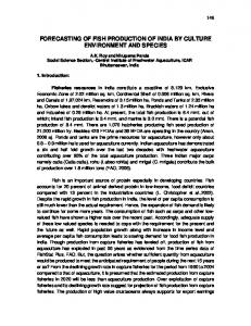
Application of the ANN model to a field data set Appropriate field data sets to test the application of the ANN model require measurements of stream flow depletions during pumping as well as data on the pumping
20
1
test and physical aquifer and stream properties. Such data sets are uncommon, but an
2
appropriate data set was found for the Winterbourne stream, which was studied as part of
3
the Lambourn Valley Pilot Scheme within the Thames Basin near Reading, Berkshire
4
(Brettell 1971). The purpose of the original study was to obtain hydrogeological data to
5
show the behaviour of the Chalk aquifer and the river system before, during, and after test
6
pumping, so as to investigate the feasibility of the proposals to augment stream flow by
7
pumping from underground. A test was carried out comparing data from this field
8
experiment with the ANN model (Walford, 2001).
9
Figure 7 (from Brettel, 1971) shows the geology of the area surrounding the
10
Winterbourne stream and the locations of the boreholes and gauging stations used for the
11
pumping tests. In the Lambourn catchment the Chalk is divided into three units: Upper,
12
Middle and Lower Chalk (Brettell 1971). Various drift deposits cover about half of the
13
solid outcrop (Figure 7). Coombe deposits or valley gravel occupy the valley bottoms
14
and lower valley slopes, having moved there by solifluction. The Chalk possesses dual
15
porosity, with effective groundwater storage being primarily within the fracture network
16
and the larger pores (MacDonald and Allen, 2001). Geophysical investigations have
17
shown that the effective aquifer is mainly in the Upper Chalk and the upper part of the
18
Middle Chalk, with significant groundwater flow occurring only in the fractures near to
19
the top of the aquifer, which generally have been enlarged by dissolution. Aquifer
20
transmissivity and storativity have a close link with topography, the aquifer properties
21
being good in valleys but significantly reducing over the interfluves (MacDonald and
22
Allen, 2001). The Winterbourne Stream is a typical chalk “bourne” or intermittent
23
stream. The point of commencement of flow changes relatively frequently, though rarely 21
1
reaches either of its extremes (Brettell, 1971). The river bed is lined with bed sediments
2
which have different hydraulic characteristics from the surrounding Chalk. The
3
conceptual model of the stream-aquifer interactions at the Winterbourne stream is
4
therefore of an unconfined Chalk aquifer overlain by valley-fill gravels.
5
Tests were carried out into flow depletion in the River Lambourn and the
6
Winterbourne Stream from 1967-1969. A test on borehole 47/3, close to the
7
Winterbourne stream, from 31 May 1967 to 20 June 1967 was chosen for analysis in the
8
present study, since this was the only year for which flow depletion was recorded for tests
9
in which the boreholes were pumped individually rather than in groups. The pumping test
10
lasted 21 days, with an average pumping rate of 7585m3/day. A continuous flow record
11
was available for Bagnor Gauging Station 2.4 km downstream of the 47/3 pumping test
12
site, and some flow data were available at gauging station D/S 47/3, 0.3 km downstream
13
of the pumping test site. The water pumped from the boreholes was carried by pipeline
14
1.6 km downstream and discharged back into the Winterbourne Stream as compensation
15
flow, so the Bagnor hydrograph shows an increase in flow during the pumping test
16
(Figure 8). To extract the flow depletion data as a result of the pumping test from this
17
flow record, it was noted that the recession limb is almost linear (excluding the period
18
over which the pumping tests were carried out). A 2nd order regression line was fitted,
19
and adjusted for the period of the pumping test to correspond to the flow value at the start
20
of the pumping test, to provide a naturalized flow. The time series of flow depletion over
21
the period of pumping test was calculated as the difference between the actual flow minus
22
the compensation flow and the naturalised flow. A similar method was used for the D/S
23
47/3 gauging site. 22
1
The parameter values used in these model simulations (Table 6) were taken from
2
Brettell (1971) and/or from unpublished data sets held by the Environment Agency,
3
Thames Region. River bed sediment conductivity was taken from infiltration
4
experiments on the Winterbourne Stream in 1968. The experiments were carried out
5
whilst the stream was dry, water being pumped down the channel and flow losses
6
between predetermined points measured. Typical values for valley gravel aquifer
7
transmissivities were found in the literature (Foreman and Sharp, 1981) and an average
8
transmissivity of 4000 m2/day was used in the model. The specific yield of the valley
9
gravel was taken as 0.25 (Freeze and Cherry, 1979). High values of transmissivity and
10
storativity for the Chalk aquifer were used, based on literature values and assuming a
11
shallow highly permeable zone of pronounced fissure development along the valley floor
12
which has been shown to act as an important conduit for feeding stream flows in similar
13
aquifers in southern England (Headworth et al., 1982). The only value which could not be
14
found was bed sediment thickness. Therefore the model was run three times: once with
15
the thickness at the mid-point in its range, 2.6m; once at its maximum (5m) and once at
16
its minimum (0.2m).
17
The output from the model for the minimum depth of bed sediment can be seen in
18
Figure 9, compared against the observed depletion at gauging stations D/S 47/3 and at
19
Bagnor. The flow depletion at Bagnor is greater than that at D/S 47/3 since it captures all
20
of the flow depletion occurring along the length of the stream. The flow depletion from
21
the model corresponds with that from Bagnor, as the flow depletion curve used in the
22
model also captures all of the flow depletion. The median and maximum values of bed
23
sediment depth produced similarly shaped curves to those with the minimum value, but 23
1
with a maximum depletion of 3100 and 1900 m3/day respectively. Only the minimum
2
value result was therefore considered further. Other than the variability of the hydrograph
3
at Bagnor, the general shape of the two field depletion curves is similar to the shapes of
4
the model output. The main difference is following the end of the pumping test (day
5
171), when the modelled depletion curves have long tails whereas observed depletion
6
drops almost immediately to zero due to the method used to calculate depletion which is
7
sensitive to small errors in the estimation of the naturalized flow. The remarkably good
8
correspondence between the simulated and observed flow depletion using independently-
9
derived parameter values demonstrates the applicability of this approach for modeling
10 11 12
realistic field conditions. CONCLUSIONS A method has been developed to assess the impacts of groundwater abstractions
13
on river flows, using a hybrid approach of numerical modeling and artificial neural
14
networks (ANN’s). The approach was based on a classification of hydrogeological
15
settings in England and Wales for the most important aquifer systems, and identification
16
and quantification of the parameters representing the factors controlling river-aquifer
17
interaction processes. Advantages of using this hybrid method are that the scope of the
18
outputs is limited only by the capabilities of the modeling system and the specification of
19
the numerical model simulations, and that the numerical modeling ensures a consistency
20
between the multiple outputs (time-series and spatial distributions of river flow depletion,
21
and groundwater levels) that may not be possible using ANN modeling alone.
22
The development of the approach presented a number of challenges which have
24
1
led to methods used to improve its efficiency and accuracy. The use of a functional
2
representation of the model outputs, implementation of an orthogonal array approach for
3
parameter value sampling, and rejection of physically unrealistic simulations, ensured
4
that the high dimensionality and large extent of the input parameter space was fully
5
spanned by the data sets used for training the ANN whilst also reducing the
6
computational workload.
7
This study was carried out in the context of decision-making for groundwater
8
abstraction licensing in England and Wales. The study has helped to inform the
9
development of operational methods currently in use by exploring the effects of
10
controlling factors on spatial distributions and time-series of river flow depletions for a
11
range of generic hydrogeological settings, and by highlighting the need to relax the
12
assumption that all water abstracted from a borehole has an impact only on the nearest
13
river. This paper has demonstrated the successful application of this approach for
14
modeling river-aquifer interactions, and its potential for modeling more complex
15
hydrological systems.
16
Acknowledgements
17
The authors thank: Prof. P.E. O’Connell for the initial suggestion of using ANN’s
18
in this context; S. Fletcher, J. Aldrick, D. Headworth, D. Burgess, P. Hulme, and other
19
Agency staff who have contributed to the study; and M. Murray who developed a
20
graphical interface for the ANN model. The work was funded by the Environment
21
Agency as R&D project number W6-046.
22
25
REFERENCES
1 2
Adams, R. and Parkin, G. 2002. Development of a coupled surface – groundwater – pipe
3
network model for the sustainable management of karstic groundwater. Env. Geol., 42,
4
513-517.
5
Aller, L., Bennet, T., Lehr, J.H., Petty, R.J., and Hackett, G. 1987. DRASTIC: a
6
standardized system for evaluating ground water pollution potential using hydrogeologic
7
settings. US Environmental Protection Agency, Ada, Oklahoma. Report No EPA/600/2-
8
87-036. 455pp
9
Brettell, E.J. 1971. Report on the Lambourn Valley Pilot Scheme, 1967-1969. Thames
10
Conservancy, Reading.
11
Birkinshaw, S.J., Parkin, G. and Rao, Z. in press. Neural Networks and Numerical
12
Models – A Hybrid Approach for Predicting Groundwater Abstraction Impacts. J.
13
Hydroinformatics.
14
Butler, J.J., Zlotnik, V.A. and Tsou, M.-S. 2001. Drawdown and stream depletion
15
produced by pumping in the vicinity of a partially penetrating stream. Ground Water,
16
39(5), 651-659.
17
Carey, M.A. and Chanda, D. 1998. Modelling the hydraulic relationship between the
18
River Derwent and the Corallian Limestone aquifer. Q. J. Eng. Geol. and Hydrogeol., 31,
19
63-72,
20
Chen, M., Soulsby, C., and Willetts, B. 1997. Modelling river-aquifer interactions at the
21
Spey Abstraction Scheme, Scotland: implications for aquifer protection. Q. J. Eng. Geol.
22
and Hydrogeol., 30, 123-136.
26
1
Conrad, L.P. and Beljin, M.S. 1996. Evaluation of an induced infiltration model as
2
applied to glacial aquifer systems. Water Resour. Bull., 32, 1209-1221.
3
Cross, G.A., Rushton, K.R. and Tomlinson, L.M. 1995. The East Kent Chalk Aquifer
4
during the 1988-92 Drought. J. Inst. of Water and Env. Man., 9, 37-48.
5
Dillon, P.J. 1983. Stream-aquifer interaction models: A review. Inst. Engrs, Australia,
6
Civil Eng. Trans., 25, 107-113.
7
Di Matteo, L. and Dragoni, W. 2005. Empirical relationships for estimating stream
8
depletion by a well pumping near a gaining stream. Ground Water, 43(2), 242-249.
9
Downing, R.A. 1993. Groundwater resources, their development and management in the
10
UK: a historical perspective. Q. J. Eng. Geol. and Hydrogeol., 26, 335-358.
11
Downing, R.A., Ashford, P.L., Headworth, H.G., Owen, M., and Skinner, A.C. 1981. The
12
use of groundwater for river augmentation. In Argent, C.R., and Griffin, D.J.H. (Eds.), A
13
Survey of British Hydrogeology 1980. Royal Society, London. pp 153 – 171.
14
Ewen, J., Parkin, G. and O'Connell, P.E. 2000. SHETRAN: a coupled surface/subsurface
15
modelling system for 3D water flow and sediment and solute transport in river basins.
16
ASCE J. Hydrologic Eng., 5, 250-258.
17
Freeze, R.A. and Cherry, J.A., 1979. Groundwater. Prentice-Hall.
18
Foreman, T.L. and Sharp, J.M. 1981. Hydraulic properties of a major alluvial aquifer - an
19
isotropic, inhomogeneous system. J. Hydrol., 53, 247-268.
20
Gray, R. 1995. An investigation of the Malmesbury Avon Catchment in the Cotswolds of
21
Southern England. In Younger, P.L. (Ed.) Modelling river-aquifer interactions. British
22
Hydrological Society Occasional Paper No. 6. pp 40-54.
23
Harbaugh, A.W. and McDonald, M.G. 1996. User's documentation for MODFLOW-96: 27
1
an update to the USGS Modular Finite-Difference Ground-Water Flow Model. US
2
Geological Survey Open File Report 96-485.
3
Hantush, M.S. 1965. Wells near streams with semi-pervious beds. J. Geophys. Res., 70,
4
2829-2838.
5
Headworth, H.G., Keating, T. and Packman, M.J. 1982. Evidence for a shallow highly-
6
permeable zone in the Chalk of Hampshire, UK. J. Hydrol., 55, 93-112.
7
Heath, R.C. 1984. Ground Water Regions of the United States. US Geological Survey
8
Water Supply Paper 2242, 78pp.
9
Hedayat, A.S, Sloane, N.J.A. and Stufken, J. 1999. Orthogonal Arrays: Theory and
10
Applications. Springer-Verlag, New York.
11
Hunt, B. 1999. Unsteady stream depletion from groundwater pumping. Ground Water,
12
37, 98-102.
13
Keating, T. 1982. A Lumped Parameter Model of a Chalk Aquifer-Stream System in
14
Hampshire, United Kingdom. Ground Water, 20, 430-435.
15
MacDonald, A.M. and Allen, D.J. 2001. Aquifer properties of the Chalk of England. Q. J.
16
Eng. Geol. and Hydrogeol., 34, 371-384.
17
McDonald, M.G. and Harbaugh, A.W. 1988. A modular three-dimensional finite-
18
difference ground-water flow model. UG Geol. Surv. Tech. Water-Resource Inv., Book
19
6, Ch, A1.
20
Modica, E., Reilly, T.E. and Pollock, D.W. 1997. Patterns and age distribution of ground-
21
water flow to streams. Ground Water, 35, 523-537.
22
Morel, E.H. 1980. The use of a numerical model in the management of the Chalk aquifer
23
in the Upper Thames Basin. Q. J. Eng. Geol. and Hydrogeol., 13, 153-165. 28
1
Owen, M. 1991. Groundwater abstraction and river flows. J. Inst. of Water and Env.
2
Man., 5, 697-702.
3
Parkin, G. and Adams, R. 1998. Using catchment models for groundwater problems:
4
evaluating the impacts of mine dewatering and groundwater abstraction. In Wheater, H. and
5
Kirkby, C. (Eds.) Hydrology in a Changing Environment, Volume II, John Wiley and Sons,
6
Chichester, pp. 269-280.
7
Prudic, D.E. 1989. Documentation of a computer program to simulate stream-aquifer
8
relations using a modular, finite-difference, groundwater flow model: US Geological
9
Survey Open-file Report 88-729.
10
Rao, Z., and Jamieson, D.G. 1997. The use of neural networks and genetic algorithms for
11
design of groundwater remediation schemes. Hydrol. and Earth System Sci., 1, 345 –
12
356.
13
Rao, Z., and O’Connell, P.E. 1999. Integrating ANNs and process-based models for
14
water quality modelling. In Proceedings of the Second Inter-Regional Conference on
15
Environment-Water, Lausanne, Switzerland, 1st – 4th September 1999.
16
Robins, N.S. 1999. Groundwater occurrence in the Lower Palaeozoic and Precambrian
17
rocks of the UK: implications for source protection. J. Inst. of Water and Env. Man., 13,
18
447 – 453.
19
Robins, N.S., Jones, H.K. and Ellis, J. 1999. An aquifer management case study - The
20
chalk of the English South Downs. Water Resour. Man., 13, 205-218.
21
Rushton, K.R. 2003. Groundwater Hydrology: Conceptual and Computational Models. J
22
Wiley, Chichester.
23
Rushton, K.R., Connorton, B.J. and Tomlinson, L.M. 1989. Estimation of the 29
1
Groundwater resources of the Berkshire Downs supported by mathematical modelling. Q.
2
J. Eng. Geol. and Hydrogeol., 22, 329-341.
3
Rushton, K.R. and Tomlinson, L.M. 1995. Interaction between rivers and the Nottingham
4
Sherwood Sandstone Aquifer. In Younger, P.L. (Ed.) Modelling river-aquifer
5
interactions. British Hydrological Society Occasional Paper No. 6. pp. 101-116.
6
Seymour, K.J., Wyness, A. and Rushton, K.R. 1998. The Fylde aquifer -a case study in
7
assessing the sustainable use of groundwater sources. In Wheater, H. and Kirkby, C. (Eds.)
8
Hydrology in a Changing Environment, Volume II, John Wiley and Sons, Chichester, pp.
9
253-268.
10
Sophocleous, M., Koussis, A., Martin, J.L., and Perkins, S.P. 1995 Evaluation of
11
Simplified Stream-Aquifer Depletion Models for Water Rights Administration. Ground
12
Water, 33, 579-588.
13
Spalding, C.P. and Khaleel, R. 1991. An evaluation of analytical solutions to estimate
14
drawdown and stream depletion by wells. Water Resour. Res., 27, 597-609.
15
Stang, O. 1980. Stream depletion by wells near a superficial, rectilinear stream. Seminar
16
No. 5, Nordiske Hydrologiske Konference, Vemladen, presented in Bullock, A., Gustard,
17
A., Irving, K., Sekulin, A. and Young, A. Low flow estimation in artificially influenced
18
catchments, Institute of Hydrology, Environment Agency R&D Note 274, WRc,
19
Frankland Road, Swindon.
20
Swain, E.D. 1994. Implementation and use of direct-flow connections in a coupled
21
groundwater and surface-water model. Ground Water, 32, 139-144.
22
Theis, C.V., 1941. The effect of a well on the flow of a nearby stream. Am. Geophys.
23
Union Trans., 22, 734-738. 30
1
van Wonderen, J. and Wyness, A. 1995. The validity of Methods used for Modelling of
2
river-Aquifer Interaction. In Younger, P.L. (Ed.) Modelling river-aquifer interactions.
3
British Hydrological Society Occasional Paper No. 6. pp. 117-129.
4
Vasiliev, O.F. 1987. System modelling of the interaction between surface and
5
groundwaters in problems of hydrology. Hydrol. Sciences J., 32, 297-311.
6
Walford, M. (2001). Testing the IGARF II (Impact of Groundwater Abstractions on
7
River Flows Phase Two) Model. Unpublished MSc dissertation, School of Civil
8
Engineering and Geosciences, University Of Newcastle upon Tyne, UK.
9
Wilson, E.E.M. and Akande, O. 1995. Simulation of Streamflow Behaviour in Chalk
10
Catchments. In Younger, P.L. (Ed.) Modelling river-aquifer interactions. British
11
Hydrological Society Occasional Paper No. 6. pp. 129-146.
12
Winter, T.C. 1984. Modelling the interrelationship of groundwater and surface water. In
13
Schnoor, J.L. (Ed.) Modeling of total acid precipitation impacts. Acid Precipitation Series
14
Vol. 9, Butterworth, London. pp. 89-119.
15
Winter, T.C. 1995. Recent advances in Understanding the interaction of Groundwater and
16
Surface-Water. Reviews of Geophysics, 33, 985-994.
17
Winter, T.C., Harvey, J.W., Franke, O.L. and Alley, W.M. 1998. Ground Water and
18
Surface Water - a single resource. U.S. Geological Survey Circular 1139. 79pp.
19
Wroblicky, G.J., Campana, M.E., Valett, H.M. and Dahm, C.N. 1998. Seasonal Variation
20
in surface-subsurface water exchange and lateral hyporheic area of two stream-aquifer
21
systems. Water Resour. Res., 34, 317-328.
22
Younger, P.L. 1987. Stream-Aquifer Interactions - A Review. NERC-WRSRU Research
23
Report 5, 115pp. Natural Environment Research Council, Water Resource Systems 31
1
Research Unit, University of Newcastle Upon Tyne.
2
Younger, P.L. 1990. Stream-Aquifer Systems of the Thames Basin: Hydrogeology,
3
Geochemistry and modelling. PhD thesis, University of Newcastle Upon Tyne. 388pp
4
Younger, P.L., Mackay, R. and Connorton, B.J., 1993. Streambed sediment as a barrier to
5
gorundwater pollution: Insights from fieldwork and modelling in the River Thames basin.
6
J. Inst. of Water and Env. Man., 7, 577-585.
7 8 9
32
1
Table 1
SHETRAN Input variables
Symbol
Description
Units
Range
D
Distance of borehole from river
m
25 – 500 or 4,000
Q
Abstraction rate
m3/day
500 – 5,000 or 10,000
tss
Time between recharge peak and start of
days
0 – 364
abstraction td
Duration of abstraction
days
1 - 365
Ka
Aquifer hydraulic conductivity
m/day
0.1 – 600
Kv
Gravel aquifer hydraulic conductivity
m/day
1 - 600
Sya
Aquifer specific yield
-
0.1– 0.5
Syv
Gravel aquifer specific yield
-
0.1– 0.5
Kb
River bed sediment hyd. conductivity
m/day
4*10-5 - 400
R
Mean annual recharge
mm/year
0 – 1000
Rs
Recharge seasonality
-
0–1
2 The maximum distance of borehole from river is 500 m for Setting 3, and 4,000 m for the 3 other settings. 4 The maximum abstraction rate is 5,000 m3/day for Setting 3 and 10,000 m3/day for the 5 other settings. 6
The input variables Ka , Sya are not used for Setting 3. The input variables Kv , Syv are not
7
used for Setting 2.
8
Recharge is applied evenly over the entire modeled area. It is represented as a sine curve,
9
with recharge seasonality being the difference between the maximum and minimum rates
10
of recharge (i.e. the amplitude of the sine function). A value of 0 is a constant recharge.
11
A value of 1 gives a maximum range of values from zero to twice the mean.
33
1
Table 2
Output variables from second Neural Network
Symbol
Description
a1
Curve shape a for flow depletion curve up to time of max depletion
p1
Curve shape p for flow depletion curve from the time of max depletion
qmax/Q
Max flow depletion/abstraction rate
tmax/td
Time of Max flow depletion/abstraction duration
a2
Curve shape a for flow depletion curve up to time of max depletion
p2
Curve shape p for flow depletion curve from the time of max depletion
qend/Q
Ratio of depletion after 25 years to abstraction rate
ar1
Curve shape a for depletion profile in river at end of abstraction
pr1
Curve shape p for depletion profile in river at end of abstraction
ar2
Curve shape a for depletion profile in river at time of max depletion
pr2
Curve shape p for depletion profile in river at time of max depletion
d
Aquifer drawdown at 5 locations at time of max depletion and 5 locations at end of abstraction (m)
dw
Drawdown in the abstraction well (m)
2
34
1
Table 3
Structure of Neural Network models
Neural Network model*
Node structure**
ANN1-1
11-7-1
ANN1-2
11-11-22
ANN2-1
9-7-1
ANN2-2
9-11-22
ANN3-1
9-7-1
ANN3-2
9-11-22
*
name refers to hydrogeological setting and model 1 (validity) or model 2
(prediction) **
input – hidden – output nodes
2
35
1
Table 4
Comparison of typical results from SHETRAN and the ANN model
Simulation
Maximum flow
Time of maximum flow
depletion (m3/day)
depletion (days)
SHETRAN
588
66
ANN
503
67
2 3 4
Table 5
Comparison of results from ANN and Stang (1980) analytical model
Simulation
Maximum flow
Time of maximum flow
depletion (m3/day)
depletion (days)
Stang analytical model ANN (Setting 3)
940
66
503
67
5 6 7
Table 6
Parameter values used to model Winterbourne Stream
Parameter Distance of borehole from river Aquifer transmissivity Valley-fill transmisivity Aquifer storage coefficient Valley-fill specific yield River width Bed sediment hydraulic conductivity Bed sediment thickness Mean annual recharge Date of peak recharge
ANN 25
Units m
1490 4000 0.1 0.25 5 0.894
m2/day m2/day m m/day
2.6, 0.2 and 5 376.55 27/02
m mm -
8
36
1
2 3
Figure 1
Schematic hydrogeological settings
4
37
1 2
Figure 2
Numerical model configuration for Settings 1 and 2
3 38
1
2 3 4
Figure 3
Variables used in processing of SHETRAN output data
5 6
39
1 2 3
Figure4
Model inputs and outputs 40
1 2 3
4 5 6 7
Figure 5
Response curves for the effect of distance of borehole from the river and abstraction duration on the maximum depletion rate (after Walford, 2001)
8 9
41
1 2
Figure 6
Conceptual models for Stang and SHETRAN solutions 42
1 2
Figure 7
Location and simplified geology of the Lambourn River (after Brettell, 1971) 43
1
2 3
Figure 8
River flow at Bagnor gauging station (after Walford, 2001)
4 5 6 7 8 9 44
1 2
Figure 9
Measured and simulated flow depletions for the Winterbourne stream
3
45