hardware in order to obtain a 3D block representation of the terrain. We test our implementation on a real model from Tupure-Carora reser- voir, Venezuela.
A Parallel Seismic Imaging and Volume Rendering in Oil Exploration German Larrazabal? and Jorge Rodriguez Multidisciplinary Center of Scientific Visualization and Computing (CEMVICC) Faculty of Sciences and Technology, University of Carabobo Valencia, Venezuela. {glarraza, jrodrigu}@uc.edu.ve
Abstract. In this work, we present an efficient parallel implementation of a depth migration RTM (Reverse Time Migration) method to obtain a seismic image. This migration technique is based on the parallel solution of the acoustic wave propagation in 2D using a finite difference scheme. We have implemented a domain decomposition on the geological section and exploit an efficient asynchronous communication between processors using MPI library. Also, we produce several axis-aligned seismic images of the terrain and apply a volume visualization technique using graphic hardware in order to obtain a 3D block representation of the terrain. We test our implementation on a real model from Tupure-Carora reservoir, Venezuela. We have applied HPC technique on a Sun Grid Cluster belongs to CEMVICC. This cluster has 16 dual AMD opteron processors Key words: Acoustic wave propagation, depth migration, domain decomposition, scientific visualization.
1
Introduction
Seismic modeling is an important part of seismic processing, because it provides the seismic answer given a terrain model. The algorithms used for seismic wave modeling to compute the seismic answer for a given terrain model, require large CPU times and memory [1]. Methods based on the wave equation [1] have been gaining popularity in recent years, because they provide more detailed and fine geological features than other conventional techniques, and also preserve the amplitude of the information. The most commonly employed numerical techniques are seismic migration and forward modeling. Migration is the last and more intensive step in the long chain of processing seismic data. Migration can be executed in time-domain as well as in depth-domain. If there are strong lateral variations of the velocity, time migration followed by time to depth conversion does not represent the reflected energy in its true subsurface position. Depthmigration is essential in these cases, because it compensates for the ray bending, ?
This work is sponsored by PDVSA Intevep S.A., CDCH–UC under No. 2005-010 and Sun Microsystems Inc. under project HPC and Grid for Oil Exploration.
2
Lecture Notes in Computer Science: Authors’ Instructions
lateral velocity pull-ups and structure. A natural advantage of depth-migration is that the output image is shown as a function of depth, and thus it can be used directly in geological interpretation. All these types of migration can be applied in 2D and 3D datasets. For obvious reasons, the resolution is far better in 3D migration, at the expense of a larger computational cost. In this work, we have developed a parallel algorithm based on reverse time migration (RTM) to obtain a seismic image. This method is based on the acoustic wave propagation. We have tested the algorithm using a slice secuence from Tupure–Carora reservoir, Venezuela. The result obtained show the good perfomance of algorithm.
2
Reverse Time Migration
The reverse time migration, is based on the full acoustic wave equation. Because the migrated image is built on a strictly spatial model of the subsurface, the product is an image in depth rather than two-way travel time. Reverse time migration can treat arbitrarily complex velocity variations and is particularly well suited for dealing with abrupt velocity changes at salt-sediment interfaces. The steps to reverse time depth migration are as follows: 1) A model of the subsurface is constructed that mimics the true spatial variation of the seismic velocity in the survey area in x, y and z. Such models are normally constructed based on initial interpretations of the seismic data, velocity analysis, and well data, if available; 2) The one-way travel times from surface source locations to a grid of subsurface points is determined by forward wave propagation or ray tracing modeling. These ”extraction” times are the times at which the reversely propagating wave fields are sampled at each depth point during the migration process; 3) A wave propagation model run is executed in the normally way forward wave propagation models are run. This is done using either the finite difference, finite element or mimetic numerical methods. The unique feature of the migration run is that instead of impulsive sources, the model surface is driven with the observed seismic traces in the reserve time order that they were recorded. This causes the observed waves to travel backwards down into the earth, towards the reflectors from which the reflections came; and 4) The migrated depth section is constructed by sampling the reversely propagating wave field at the extraction time at each subsurface point. The extraction time associated with a depth point corresponds to the time at which a reflection refocuses at the true reflector position. 2.1
Forward wave propagation model
The mathematical model implemented in this work is based on [2] [3]. We consider the acoustic wave equation in heterogeneous media. This equation is obtained from Euler’s relation and continuity equation: � � ∂2P → 1− → 2− ∇P = δ (r) src (t) . (1) − ρc ∇ ∂2t ρ
Paralle Seismic Imaging and Volume Rendering
3
where v is the particle velocity, P is the acoustic pressure, ρ is the density, and c is the wave velocity on the medium. The equation is modified to include the source function src(t) by adding a term to the right–hand side. We use the Dirac delta function (δ(r)) to position the source in space and use the source function src(t) to define its characteristic shape in time. If we solve equation (1) numerically with an explicit integration method the criterion of stability √ for a heterogeneous media√is (c∆t)/(∆x) ≤ (1/ 2), where c is the maximum velocity in the media and 2 results from the model dimension, 2D in this case. According to Alford et al. [4], the following relation will be used in order to minimize the dispersion in the model is max(∆x, ∆z) ≤ (λdominant /10), where the term λdominant represents the dominant wavelength in the model. We need to define absorbing boundary conditions in order to avoid undesirable reflection. We use the function of weights presented by Cerjan et al. [5]. A source function is required to generate the seismic wave. The method used in this work will be to simulating a dynamite explosion to generate the seismic waves. We use a Ricker function. We now apply a second-order difference scheme to the wave equation (1). We use centered differences to approximate the second derivative with respect to time and space. We use boundary conditions presented in [6].
3
Parallel Algorithm and Volume Rendering
The parallel implementation of the algorithm is based on domain decomposition using MPI. Domain decomposition involves assigning sub-domains of the computational domain to different processors and solving the equations for each subdomain concurrently. Here, the domain is partitioned in z–direction. Once the RTM has been achieved for several axis-alligned 2D sections, a volume dataset is obtained and a direct volume rendering technique is applied in order to visualize a 3D representation of the terrain. The volume rendering technique applied is based on a ray-casting algorithm, using the low-albedo integral for the opacity composition. Also, a graphic hardware assited implementation can be used to achieve the volume visualization depending on the size of the volume dataset generated.
4
Test Problem and Performance
The hardware platform is a Sun Grid Cluster machine with 16 Opteron 248 dual nodes, having a total of 32 processors. The parallel RTM code was developed in ANSI C applying HPC techniques. We have used our parallel RTM algorithm to tune the seismic acquisition parameters of a theoretical-geological secuence section of Tupure–Carora reservoir. We have 500 sections cross–line. Each one of this, has 119,200 meters in–line and 22,400 meters in depht. We have used 2,384 gathers/shots on each cross–line section. The simulation time was 5 seconds and we use 60 Hz. of maximal frequency. The parallel CPU time was 41 minutes and the time rendering was 8 seconds. The figure 1(a), we can observe the 3D velocity uniform model. The seismic image obtained can be observed in the figure 1(b).
4
Lecture Notes in Computer Science: Authors’ Instructions
a) 3D Velocity model.
b) Imaging after migration.
Fig. 1. 3D Geologycal model of Tupure Carora reservoir, Venezuela.
5
Conclusions
In this work, we have presented an efficient parallel implementation of a depth migration RTM (Reverse Time Migration) method to obtain a seismic image. We have implemented a domain decomposition on the geological section and exploit an efficient asynchronous communication between processors using MPI library. Also, we have produced several axis-aligned seismic images of the terrain and applied a volume visualization technique using graphic hardware in order to obtain a 3D block representation of the terrain. We have tested our implementation for a real model from Tupure-Carora reservoir, Venezuela. We have applied HPC techniques on a Sun Grid Cluster belongs to CEMVICC.
References 1. Phadke, S., Bhardwaj, D. and Yerneni, S., (1998), ”Wave equation based migration and modelling algorithms on parallel computers”, Proceedings of SPG98, 55–59. 2. Bordin R., (1995) ”Seismic wave propagation modeling and inversion”, Computational Sciences Educational Project, Stanford University, USA. 3. Bordin R. and Lines L. (1999), ”Seismic modeling and imaging with the complete wave equation”, Society of Exploration Geophysicists (SEG). 4. Alford R. M., Kelly K. R. and Boore D. M. (1974). ”Accuracy of finite–difference modeling of the acoustic wave equation”, Geophysics, 39, 834–842. 5. Cerjan C., Kosloff D., Kosloff R. and Reshef M. (1985). ”A nonreflecting boundary condition for discrete acosutic and elastic wave equations”, Geophysics, 50, 705– 708. 6. Reynolds A. C. (1978). ”Boundary conditions for the numerical solution of wave propagation problems”, Geophysics, 43, 1099–1110.