1
A Parameterized T-S Digital Fuzzy Logic Processor: Soft Core VLSI Design and FPGA Implementation K. M. Deliparaschos, S. G. Tzafestas Intelligent Robotics and Automation Laboratory School of Electrical and Computer Engineering National Technical University of Athens Zographou Campus, Athens, GR 157 73
[email protected],
[email protected] Abstract: Fuzzy Logic (FL) was developed by Zadeh to deal with the uncertainty involved in decision making and system modeling and control of real–life systems, and is an extension of the two– valued logic defined by the binary pair {false, true} or {0,1} to the entire continuous interval [0,1] of logic values between false=0 and true=1. The purpose of this paper is to design and implement a zero-order Takagi-Sugeno (T-S) parameterized digital fuzzy logic processor (DFLP), in which only the active rules (i.e. rules that give a non–null contribution for a given data set) are considered, at high speed of operation, without significant increase in hardware complexity. The DFLP discussed in this paper achieves an internal core processing speed of at least 100 MHz, and based on the chosen parameters is featuring four 12-bit inputs and one 12-bit output, with seven trapezoidal shape membership functions per input and a rule base of up to 2401 rules. The proposed architecture was implemented in a Field Programmable Gate Array (FPGA) chip with the use of a very high-speed integrated-circuit hardware-description-language (VHDL) and advanced synthesis and place and route tools. Key-Words: - Fuzzy Logic processor (FLP), digital FLP (DFLP), Takagi-Sugeno controller, field programmable gate array (FPGA) chip, very high-speed integratedcircuits description language (VHDL).
1. INTRODUCTION Fuzzy chips are distinguished into two classes depending on the design techniques employed: digital and analog. The first fuzzy chip was reported in 1986 at AT&T Bell Laboratories (Murray Hill, NJ) [4]. The digital approach originated from Togai and Watanabe’s paper [4] and resulted in some interesting chips [5][6]. Other digital architectures were reported in [11][12]. Analog chip approaches begun with Yamakawa in [7][8]. This paper presents the design of a parameterized digital fuzzy logic processor (DFLP). By the term parameterized we mean that the DFLP facilitates scaling
and can be configured for different number of inputs and outputs, number of triangular or trapezoidal fuzzy sets per input, number of singletons per output, antecedent method (t-norm1 , s-norm2 ), divider type, number of pipeline registers for the various components in the model. This parameterization enables the creation of a generic Fuzzy Controller (FC) Core than can be used to produce fuzzy processors of different specifications without the need of redesigning the FC Core from the beginning. The fuzzy logic processor architecture assumes overlap of two fuzzy sets between adjacent fuzzy sets and requires 2n clock cycles (input data processing rate), where n is the number of inputs, since it processes one active rule per clock cycle. The architecture of the design allows one to achieve a core frequency speed of 100 MHz, while the input data can be sampled at a clock rate equal to 1/2n of the core frequency speed (100 MHz), while processing only the active rules. To achieve this timing result the latency of the chip architecture involves 11 pipeline stages each one requiring 10 ns. The proposed DFLP is based on a simple algorithm similar to the Takagi-Sugeno of zero-order type inference and weighted average defuzzification method, and based on the chosen parameters employs four 12-bit inputs and one 12-bit output, with up to 7 trapezoidal or triangular shape membership functions per input with a degree of truth resolution of 8 bits and a rule base of up to 2401 rules.
2. FUZZY LOGIC 2.1 Theory of fuzzy sets Fuzzy Set Theory was developed by Lotfi Zadeh in 1965 [1], where he introduced the fuzzy set concept. Zadeh, has extended the two value logic, defined by the binary pair {0, 1}, to the whole continuous interval [0, 1], introducing a gradual transition from falsehood to truth. A “crisp” set is closely related to its members, such that an item from a given universe of discourse is either a member (1) or not (0). Zadeh, suggested that many sets have more than a yes (1) or not (0) crisp criterion for membership and he proposed a grade of membership (µ) in the interval [0, 1], such that the decision whether an 1 2
t-norm: ┬min(a,b)=min{a,b}, ┬prod(a,b)=a·b s-norm: ┴max(a,b)=max{a,b}, ┴sum(a,b)=a+b-a·b
2
element (x) belongs or not to a set (A) is gradual rather than crisp (or binary). In other words, fuzzy logic replaces “true or 1” and “false or 0” with a continuous set of membership values ranging in the interval from 0 to 1. If U defines a collection of elements denoted by x, then a fuzzy set A in U is defined as a collection of ordered pairs: A = {(x, µA(x)) | x∈U} The elements (x) of a fuzzy set are said to belong to a universe of discourse, U, which effectively is the range of all possible values for an input to a fuzzy system. Every element in this universe of discourse is a member of the fuzzy set to some degree. The function µA(x) is called a membership function and assigns a degree of truth number in the interval [0, 1] to each element of x of U in the fuzzy set A. 2.2. The Takagi-Sugeno Method The DFLP proposed in this paper is based on the T-S zero-order type fuzzy model [2][3]. It is well known that the T-S fuzzy model can provide an effective representation of complex nonlinear systems in terms of fuzzy sets and fuzzy reasoning. The T-S method is actually quite simple as a method, leads to fast calculations and is relatively easy to apply. Moreover, a fuzzy processor based on the T-S method provides a good trade-off between the hardware simplicity and the control efficiency. In the T-S inference rule, the conclusion is expressed in the form of linear functions. T-S MIMO rules have the following form: Rule Ri: IF x1 IS Ai1 AND x2 IS Ai2 AND… AND xn IS Ain THEN yi1 AND yi2 AND… AND yil where yij = ci0j + ci1j x1 + … + cinj xn i=1,2,…,m where m is the total number of rules, xk, k=1,2,…,n represents the kth input variable, Aik is the input fuzzy sets, yij, j=1,2,…,l represents the jth output variable of the ith rule, and cikj are all constants. The above rule is linguistically (logically) equivalent to a number of MISO rules, such as: Rule Ri: IF x1 IS Ai1 AND x2 IS Ai2 AND… AND xn IS Ain THEN yi1 Rule Ri: IF x1 IS Ai1 AND x2 IS Ai2 AND… AND xn IS Ain THEN yij The logical “AND” in the consequent of the MIMO rule still exists in the MISO rules case since in the two fuzzy inferences the one set of rules is true “AND” another is true [20]. A zero-order model arises (simplified T-S functional reasoning), if now we only use the constant ci0j at the output and therefore yij=ci0j (singleton outputs). In the T-S model, inference with several rules proceeds as usual, with a firing strength associated with each rule, but each output is linearly dependent on the inputs.
The output from each rule is a moving singleton, and the deffuzified output is the weighted average of the contribution of each rule, as shown in the following equation: m
yj =
wi y ij ∑ i =1 m
wi ∑ i =1
where wi is the weight contribution of the left part of the ith rule and for AND method connection is given by n
n
w = ∏ µ A ( xk ) or w = min µ A ( xk ) i
i
i
k =1
i
k =1
k
k
The T-S mechanism is illustrated in Figure 1: Consequent (singleton MF) ci
Fuzzification of Input 1
x1
Inference mechanism
Antecedent connection via T-norms (conjunction “and”) or T-conorms (disjuntion “or”)
Fuzzification of Input n
Firing strength (θi) Rule i Rule 1
Implication (Product Method)
Rule inference (θi *ci )
Aggregation
Defuzzification
y1
xn
Figure 1: T-S mechanism. 2.3. DFLP Characteristics In this section, the characteristics of our DFLP are presented based on the chosen (generic) parameters (defined on a VHDL package file) for the parameterized FC CORE. These are summarized in Table 1 and Table 2 respectively. Parameters (VHDL generics) ip_no ip_sz op_no op_sz
Value 4 12 1 8
FS_no dy
7 8
sel_op
0
div_type Path Synchronization Registers psr1_no psr2_no psr3_no psr3_no Component Pipeline Registers cpr1_no cpr2_no cpr3_no cpr4_no cpr5_no cpr6_no cpr7_no cpr8_no cpr9_no
0
Generic Description number of inputs input bus width (bits) number of outputs output bus width (bits) number of membership functions (same for all inputs) dy degree of truth width antecedent method connection: 0 : min, 1: prod, 2: max, 3: probor divider model type 0: restoring array, 1 : LUT reciprocal approximation [19]
1 4 2 0
Signal Path Route ip_set -> psr1_no -> trap_gen_p s_rom ->psr2_no-> mult s_rom ->psr3_no-> rul_sel_p cpr5 ->psr-> int_uns
1 1 3 0 2 2 2 0 3
Component (Entity) Name addr_gen_p cons_map_p trap_gen_p rule_sel_p minmax_p mult int_uns int_sig div_array
3 r_in
U2
control_logic_p clkd ready_in clkm rst_n ready_out
**truncat ed to 12 bits
IF* U13
div_ppa divd op divs
U7
*
clkdv clkx rst_n
CPR9 R2 div_array X op Y
Divider type selection
1
CPR7 CPR5
16
Defuzzyfication Area 8
CPR4
CPR2
I nference Engine Area
PSR3
U4
U11
andor_meth_p ip_data op_data
s_rom_p addr data
16
Note: CPR{1,9}, PSR{1,3} Register delays (R{1, 2}), clocked by clkx. All reset by rst_n.
U5
mult x_signed y
8 x_unsigned
CPR6
21
PSR2
Top St ructural DFLP Parameterized Soft Core Design (U1)
int_uns clk rst _n y x clear clkx rst_n
U12
int_sig clear x y clk rst_n
12
32
12
32
U3
U10
cons_map_p addr_in addr_out
rule_sel_p sel op_dat a ip_dat a
16
12
CPR1
CPR3
32
1
addr_gen_p ip_data int_zer clk rst_n gen_addr
12
ip2 ip3
R1 ip1
Fuzzyfi cation Area
U9
trap_gen_p mf_param alpha_val ip_data
U8
48
48
ip0
rst
160
PSR1
U1
rst
clk
ars_p f s_start_addr ip_data clkx rst _n
U0
mf_rom_p data addr
U2
32
12
clkdv clkx rst _n
3.1 DFLP Architecture The present DFLP architecture is shown in Figure 2. The architecture is mainly broken in three major hierarchical blocks: “Fuzzification”, “Inference” and “Defuzzification”. The “CPR” blocks on the figure indicate the number of pipeline stages for each component (component pipeline registers), the “PSR” blocks indicate the path synchronization registers, while the “U” blocks represent the different components of the DFLP. The component identified as DCM is the Digital Clock Manager and is one of four components available in the specific FPGA library chosen (Spartan-3 1500-4FG676) [15]. The latter accepts the FPGA board (Memec 3SMB1500) clock (clk) of 75 MHz and is configured to generate a divided clock signal (clkdv) of 75 MHz/12=6.25 MHz and a multiplied clock signal (clkfx) which is 6.25·16=100 MHz for the DFLP Core operation. It should be mentioned here that the above frequency values can vary by changing the DCM generic parameters. A control logic component (control_logic_p) is implemented on the top structural entity (binds FC Core, DCM, R1, R2 and control logic) of the design that provides two signals named “ready_in” and “ready_out”, which are used to provide input and output data-ready
1
12
25
12
DCM
This section provides an analytical description of the various hierarchical blocks of the DFLP architecture, and explains how these blocks are designed in a parameterized fashion to result in a fully parametric processor core.
clk
3. DFLP HARDWARE IMPLEMENTATION
25
21
MIN (T-norm operator implemented by minimum) PROD (product operator) 2 Weighted average
Table 2: DFLP characteristics
12
12**
CPR8 U6
2401 Singleton type 8 bit 2401 (number of fuzzy sets number. of inputs)
Top structural design on FPGA Chip
Implication method MF overlapping degree Defuzzification method
Takagi-Sugeno zero-order type 4 12 bit 1 12 bit 7 Triangular or Trapezoidal shaped per fuzzy set 8 bit
Clock management
Fuzzy Inference System (FIS) type Inputs Input resolution Outputs Output resolution Antecedent Membership Functions (MF’s) Antecedent MF degree of truth (α value) resolution Consequent MF’s Consequent MF resolution Maximum number of fuzzy inference rules AND method
op
The necessary parameters are assigned on the generics on the entity definition of every parameterized VHDL component in the design hierarchy. On the same VHDL package file, the number of pipeline stages for every functional block in the design as well as path synchronization registers is defined.
r_out
signals for handshaking with external devices.
IF GENERATE Stat ement
Table 1: DFLP Soft Core chosen parameters
4
Figure 2: DFLP Parameterized Soft CORE architecture. 3.2. Active Rule Selection block Instead of processing all the rule combinations for each new data input set, we have chosen to process only the active rules, i.e. those rules that give a non null contribution to the final result. Dealing with the above problem and given the fact that the overlapping between adjacent fuzzy sets is of order 2, we have implemented an active rule selection block (ars_p) to calculate the fuzzy set region in which the input data corresponds to. As a result, for the 4-input DFLP with 7 membership functions per input, instead of processing all 2401 rule combinations in the rule base, only 16 active rules remain that need to be taken into account. Fig. 3, illustrates the fuzzy set (FS) coding used for the inputs (ip0,…,4) , as well as the FS area split up that occurs by repeatedly comparing the four input data values (ip0,…,4) with the rising start points (rise_start0,…,4) of the fuzzy sets. Since we assume overlapping of two fuzzy sets between adjacent fuzzy sets, it is obvious that the comparison of the 1st and 2nd FS is not necessary, since the initial FS pair is always the 1st and 2nd and we only shift right to the next FS pair when the rise_start (rs) of the 3rd FS is exceeded. The FS section transition is depicted in Figure 3 as line type named ‘change in ars’. Generally, FS_start_addr0,…,4 denotes the active FS pair and its output range is from 0 to 5 in this case. change in ars
dy 0 Selecting ars FS regions for ip0
MF0
MF1
MF2
MF3
MF4
MF5
(2)
(3)
(4)
MF6
ip0 (FS_start_addr)
(0)
(1)
(5)
Figure 3: FS coding ars_p address regions. An analytical block diagram for the parameterized ars_p block is shown in Figure 4. In the same figure a snapshot of the architecture of the ars_p block is provided, showing the VHDL code style followed to achieve parameterization is illustrated. The parameterization is mainly achieved by making use of the generate statement available in VHDL and use of generics in the entity to define the parameters of the block.
ars_p Parameters ROM Array 0
0 rs4
1 r s3
r s2
rs1
FS_no-2 rs0
1
rs4
r s3
r s2
rs1
rs0
ip_no-1
rs4
r s3
r s2
rs1
rs0
ip_data
FS_start_addr
ars_p
Ip_no*ip_size
ip_no*log2(FS_no- 1)
ip_size (FS _no-2)*ip_size
FS_start_addr
ip_data ip_no*ip_size
ars_p Combinatorial logic
ip_size ip_size
log2(FS_no-1)
ip_no*log2(FS_no-1)
log2(FS _no-1)
ip_size
log2( FS_no-1)
architecture rtl of ARS _p is begin - - ARCHITECTURE rtl A : for i in 0 to ip_no-1 generate signal sel : std_logic_vector (ip_sz -1 downto 0) ; signal addr _out : std_logic_vector(log2(FS_no-1) -1 downto 0);
Shown for one input ip_data rs0
begin - - GENERATE -- select sel '1');
e d
[31:24]
[3:0]
op_data[31:0]
[2]
1*8
e d e d
[7:0]
e d
A.2.un61_x_dec A.0.x_dec_2[7:0]
0*8 [1] [15:8] [1]
1*8
e d e d
[7:0]
e d
A.1.un39_x_dec A.0.x_dec_1[7:0]
0*8 [0] [7:0] [0]
A.0.un15_x_dec
1*8
e d e d
[7:0]
e d
A.0.x_dec[7:0]
Figure 11: Rule selector VHDL code and synthesis result (RTL view).
More specifically, in reference to Figure 11, when the antecedent of a rule is not active, it will not contribute to the final weight of the rule. Provided that the weight contribution of the rule (theta value) is extracted using the min operator, we can ignore the alpha value of the chosen antecedent by setting it to its maximum value which in our case for dy=8bit degree of truth resolution (unsigned number since alpha value, α∈ R+) is 28-1=255. Finally, if all rule antecedents are inactive, at least one alpha value must be set to a minimum value, so that the weight
rst_n
clk clear [24:0] 0*25
0 1
[24:0] [24:0]
prev_ip.x_p1_3[24:0] rst_n x[20:0]
D[24:0]
Q[24:0] R
[24:0]
[20] [20] [20] [20] [20:0]
[24:0]
+
[24:0] [24:0]
y[24:0]
un4_y_c[24:0]
x_p1[24:0]
[20:0]
Figure 12: Integrator block and RTL synthesis result
3.8. Multiplier blocks. The Spartan 3 family of FPGA devices [15] used to implement the proposed architecture provides embedded multipliers, where their number varies depending on the family code. At present, we have used a Spartan 3 1500 FPGA providing a total of 32 dedicated multipliers. The input buses to the multiplier accept data in two’s-complement form (either 18-bit signed or 17-bit unsigned). One such multiplier is matched to each block RAM on the die. The close physical proximity of the two ensures efficient data handling. The multiplier is placed in a design using one of two primitives; an asynchronous version called MULT18X18 and a version with a register at the outputs called MULT18X18S. In the present design the latter multiplier type was used since it leads to better timing results. 3.10. AND/OR method block This block simply implements different intersection/union (AND/OR) methods for the antecedent connection. It is fully parameterized with respect to the number and resolution of input antecedents and method selection. The block implements the following norms (sel_op = 00 for min1, 01 for prod1, 10 for max2, 11 for probor2 (probabilistic OR or algebraic sum). 3.11. Divider block Division remains one of the hardware consuming operations. Several methods have been proposed [13]. These methods which target on better timing results, usually start with a rough estimation of the Reciprocal = 1/ Divisor and follow a repetitive arithmetic method, where the number of repetitions depends on the precision
7
difference of the reciprocal with the desirable division precision. A similar method is followed here, but the reciprocal precision is calculated in such a way that it is the minimum possible for achieving the desired precision at the divider output without the need of any repetitions. This way, the division is simplified to a multiplication operation between the reciprocal estimation and the dividend. At this point it has to be mentioned that we treat the minimum reciprocal precision estimation based on all possible data values that occur from the weighted average defuzzification method: m
op =
m
bit l ength of reci procal approximation2
round Divide3
M ATLAB Functi on
theta value bi t length
random theta (andor_m eth_p)
divd (i nt_sig)
Product1
Di vi de1
500
2000
2500
3000
3500
4000
4500
[0] [1] [2] [3] [4] [5] [6] [7] [8]
aproxim ati on
[9] [10] [11]
error
Subtract1
1500
The divider block (div_ppa) synthesis result is shown in Figure 16, where the component named recip_lut_p is the ROM that holds the reciprocal LUT contents (Figure 15).
2^0 Rounding Operation1
1000
Figure 15: Reciprocal LUT contents.
real Constant
2^22 bit length of reciprocal approxi mati on1
2 1.5
Roundi ng Operation2
Product2
fl oor di vs (i nt_uns)
3 2.5
0
2^22
8
4 3.5
0
wi ∑ i =1
M ATLAB Functi on
x 10
0.5
The precision of the reciprocal was estimated at 22 bit using the Simulink model shown in Figure 13: 12
6
4.5
1
wi yij ∑ i =1
singleton random si ngletons (s_rom _p) bi t length
very effective as it increases the reciprocal memory size and leads to bigger multiplication, we have chosen to add two extra circuits to detect these cases. The reciprocal memory contents are shown on the graph of Figure 15:
op2
Product3
divs[11:0]
[11:0]
un3_op
Divi de2
divd[24:0] 1
[0] [1] [2] [3] [4] [5]
Scope2 Constant1
2^12
mod floor
Math divs bi t length Function2
Divide1
recip_rom
1
To Workspace1
2^22 bi t length of reciprocal approxi mati on1
Memory
[24:0]
Figure 13: Reciprocal precision estimation and reciprocal ROM generation Simulink models.
The output error for the model considered above is shown in Figure 14:
[6] [7] [8] [9] [10] [11]
un16_op
un7_op
e d
1*12
e d
[33:22]
e d
[11:0] op[11:0] [11:0]
op[11:0]
[24:0] =0 [21:0]
[11:0]
[11:0]
*
+-
[47:0]
op_tmp[47:0]
recip_lut_p Addr[11:0]
Data[21:0]
[21:0]
U
Figure 16: Divider block RTL synthesis result view
1 0.8
4. DESIGN FLOW FOR DFLP
0.6 0.4 0.2 0 -0.2 -0.4 -0.6 -0.8
0
100
200
300
400
500
600
700
800
900
1000
Figure 14: Output error.
Figure 14 clearly shows that the resulting error is not greater than 0.8 and the output is valid for the desired 12 bit output. This error is practically rounded since the output is scaled down to 12 bits. The “divide by zero” case has no practical value since it happens when all the theta values are zero, or when the antecedents of the rules have been disabled (by the rule selector) leading to no contributing consequences (from the s_rom_p). The latter case consequently means that for the present input data set, there are no defined rules. Thus we set the output to minus one (1/0≡-1). Adding the case where divd/1=divd, increases the reciprocal memory (reciprocal LUT block in Figure 2) word length from 22 to 23 bit. Since this is not
This section presents the design flow (Figure 17) in a topdown manner, followed in our DFLP design. In a top-down design, one first deals with the specification and then with the design of the circuit functionality. The starting point of the design process is the system level modeling (Simuling model) of the proposed DFLP. The Simulink model enabled us to evaluate the proposed DFLP, and to extract valuable test vector values to be used later for RTL and timing (VITAL) simulation. The VHDL language was used for the description of the circuit in RTL (Register Transfer Level). Special attention was paid on the coding of the different components, since we aimed on writing a fully parameterized code. The DFLP can be parametric in terms of the number of available inputs and their resolution in bits, number of fuzzy sets per input and resolution of alpha value in bits, number of outputs and bit size of the output resolution, antecedent connection method, divider type, as well as in terms of the number of pipeline stages each block has. The DFLP presented here uses the generic parameters chosen in Table 1. A VHDL package stores the above generic parameters together with the number of
8
necessary pipeline stages for each block. An RTL simulation was performed to ensure the correct functionality of the circuit. Next, logic synthesis [14] was done, where the tool first creates a generic (technology independent) schematic on the basis of the VHDL code and then optimizes the circuit to the FPGA specific library chosen (Spartan-3 15004FG676). At this point, area and timing constraints and specific design requirements must be defined as they play an important role for the synthesis result. Next, the Xilinx place and route (PAR) [14] tool accepts the input netlist file (.edf), previously created by the synthesis tool and goes through the following steps. First, the translation program, translates the input netlist together with the design constraints to a Xilinx database file. After the translation program was run successfully, the map program maps the logical design to the Xilinx FPGA device. Finally the PAR program accepts the mapped design, places and routes the FPGA, and produces the output for the bitstream (BitGen) generator. The latter program receives the placed and routed design and generates a bitstream (*.bit file) for Xilinx device configuration. Before programming the FPGA file, a VITAL simulation was performed to ensure that the circuit meets the timing requirements set and works correctly. Test Vector Generation
Design Specifications
DFLC System Modelling
Synthesis Optimization
Place & Route Optimization
Synthesis Constraints
Place & Route Constraints
Logic Synthesis
Place & Route
Functional Optimization
VHDL RTL Description
RTL Simulation Mentor Modelsim
Mathworks Matlab, Simulink
Debugging
Results OK no
yes
Synplicity – Synplify
Area & Timing Report
Xilinx – ISE
VITAL Simulation
Results OK
yes
“.bit” File
no no Constraints Met
yes
Debugging
FPGA Device Implementation
Figure 17: Design Flow Map.
5. RESULTS Figure 18 shows the data flow for all the signals specified in Figure 2. A new input data set is clocked on the rising edge of the clkdv_out clock, with 1/16 the frequency of the clkfx_out clock, providing the necessary time (16 algorithmic clock cycles) for the Address Generator (pipeline stage, cpr1) to generate the signals corresponding to all active rules (2nd-17th clock cycles). Here, we remind that by using the ars_p block we effectively identify and process 16 active rules per clock cycle instead of 2401 [8]. The Trapezoidal Generator (trap_gen_p) block requires three pipeline stages (cpr3) to compute the α values of the membership functions. The computation occurs while the system addresses and reads the Singletons ROM. Two clocks later (cpr5), after the rule selection (rule_sel_p) and the Minimum operator (andor_meth_p) have taken place for the pair of the active rules, their θ values (MIN operation on the α values) along with their consequents and the signal for zeroing the integrators become available for the Inference and Defuzzification part. The rules implication result (mult), occurs two clocks later along
with the addition of the θ values. In the next clock, the sum of the implications is computed. During that time the unsigned integrator (div_uns) outputs the divisor value (cpr7), while the dividend is computed by the signed integrator (div_sig), three clocks later (cpr9) the LUT reciprocal division estimation (div_ppa) becomes available. The total data processing time starting from the time a new data set is clocked at the inputs until it produces valid results at the output requires a total latency of 27 pipe stages or 270 ns which is analyzed in 16 algorithmic clock cycles (see the Address Generator - section 3.3) and 11 clock cycles due to pipelining (Table 1). This effectively characterizes the throughput data processing rate of the system (a new input data set can be sampled every 16 clocks or 160 ns), while the internal clock frequency operation of the DFLP Core is 100 MHz or 10 ns period. Along with the proposed DFLP architecture, a modified model with LUT based MF Generator blocks, instead of arithmetic based, has been implemented which is not presented in this paper. The latter DFLP model achieves a better timing result with the same levels of pipelining, but with significant increase in FPGA area utilization compared to the presented model. Moreover, it is obvious that since the MF’s are ROM based any type and shape could be implemented.
9
We have managed to design a parameterized and amenable to scaling, digital fuzzy logic processor (DFLP) soft core that processes only the active rules for a given input data set, thus increasing substantially the overall input data processing rate of the system. The soft core model is parametric in terms of the different number of inputs and outputs, number of triangular or trapezoidal fuzzy sets per input, number of singletons per output, antecedent method connection, divider model type, and number of pipeline registers for the individual components in the hierarchy. The parameterized DFLP Core allows the creation of various fuzzy processors without the need of recoding the RTL components description. Two DFLP architectures based on the selected parameters (Table 1) were implemented; one with arithmetic -and one with LUT- based membership function generators (not described in this paper). The parameters in Table 1 were selected so as to create the fuzzy controller required for balancing control of the Pendubot inverted pendulum [18]. A laboratory experiment is inprogress for the evaluation of the capabilities of this controller. The results of this evaluation will appear elsewhere.
cpr7
cpr9
6. CONCLUSIONS AND FUTURE WORK
cpr5
REFERENCES
cpr3
[1]
cpr1
[2]
[3]
[4]
Figure 18: Pipeline structure data flow.
The resources employed on the FPGA device (xc3s1500) for the DFLP model (based on the parameters of Table 1) are summarized in Table 3: Logic Utilization Number of Slice Flip Flops: Number of 4 input LUTs: Logic Distribution: Number of occupied Slices: Number of Slices containing only related logic: Number of Slices containing unrelated logic: Total Number 4 input LUTs: Number used as logic: Number used as a route-thru: Number used as 16x1 ROMs: Number of bonded IOBs: Number of Block RAMs: Number of MULT18X18s: Number of GCLKs: Number of DCMs:
Used Available Utilization 725 26,624 2% 2,195 26,624 8% 2,054
13,312
15%
2,054
2,054
100%
0
2,054
0%
3,635 2,195 32 1,408 64 3 4 3 1
26,624
13%
[5]
[6]
[7]
[8] 487 32 32 8 4
13% 9% 12% 37% 25%
Table 3: xc3s1500 FPGA Utilization for DFLP Model.
[9]
L. A. Zadeh, “Fuzzy Sets”, Inf. and Control, Vol.8, pp.338-353, 1965. T. Takagi & M. Sugeno, “Derivation of Fuzzy Control Rules from Human Operator's Control Actions”, Proc. of the IFAC Symp. on Fuzzy Inform., Knowledge Represent. and Decision analysis, pp.55-60, July 1983. T. Takagi & M. Sugeno, “Fuzzy Identification of Systems and Its Application to Modeling and Control”, IEEE Trans. Syst. Man & Cybern., Vol.20, No.2, pp.116-132, 1985. M. Togai, H. Watanabe, “A VLSI Implementation of a Fuzzy Inference Engine: Toward an Expert System on a Chip”, Inform. Sci., Vol.38, pp.147-163, 1986. H. Watanabe, W. D. Dettloff, K. E. Yount, “A VLSI Fuzzy Logic Controller with Reconfigurable, Cascadable Architecture”, IEEE J. Solid-State Circuits, Vol.25, No.2, pp.376-382, Apr. 1990. K. Shimuzu, M. Osumi, F. Imae, “Digital Fuzzy Processor FP-5000”, Proc. 2nd Int. Conf. Fuzzy Logic Neural Networks, Iizuka, Japan, pp.539-542, July 1992. T. Yamakawa and T. Miki, “The Current Mode Fuzzy Logic Integrated Circuits Fabricated by the Standard CMOS Process”, IEEE Trans. Comput., Vol.C-35, pp.161-167, Feb. 1986. T. Yamakawa, “High Speed Fuzzy Controller Hardware System: The mega-FLIPS Machine in Fuzzy Computing”, Inf. Sci. M. M. Gupta and T.Yamakawa, Eds. Amsterdam, The Netherlands: Elsevier, 1988, Vol.45, No.1, pp. 113-128. A. Gabrielli, E. Gandolfi, “A Fast Digital Fuzzy Processor”, IEEE Micro, Vol.17, pp.68-79, 1999.
10
[10] C. J. Jiménez, A. Barriga. S. Sánchez-Solano, “Digital Implementation of SISC Fuzzy Controllers”, Proc. Int. Conf. on Fuzzy Logic, Neural Nets and Soft Computing, pp.651-652, Iizuka, 1994. [11] M. J. Patyra, J. L. Grantner, K. Koster, “Digital Fuzzy Logic Controller: Design and Implementation”, IEEE Trans. Fuzzy Syst., Vol.4, No.4, pp.439-459, Nov. 1996. [12] H. Eichfeld, T. Künemund, M. Menke, “A 12b GeneralPurpose Fuzzy Logic Controller Chip”, IEEE Trans. Fuzzy Syst., Vol.4, No.4, pp.460-475, Nov. 1996. [13] Derek Wong, Michael Flynn, “Fast Division Using Accurate Quotient Approximations to Reduce the Number of Iterations”, IEEE Trans. Comp., Vol.41, No.8, Aug. 1992. [14] D. L. Perry, “VHDL: Programming by Example”, 4th ed. McGraw-Hill, 2002. [15] Xilinx, “Spartan-3 FPGA Family: Complete Data Sheet”, DS099 Dec. 24, 2003. [16] S.G. Tzafestas and A.N. Venetsanopoulos (eds), “Fuzzy Reasoning in Information”, Decision and Control Systems, Kluwer, Dordrecht, 1994. [17] S.G.Tzafestas (ed.), “Soft Computing in Systems and Control Technology”, World Scientific, Singapore London, 1997. [18] Spong, M.W., and Block, D.J., “The Pendubot: A Mechatronic System for Control Research and Education,” 34th IEEE Conf. on Decision and Control, pp. 555-556, New Orleans, Dec., 1995. [19] K. M. Deliparaschos, F. I. Nenedakis and S. G. Tzafestas, “A Fast Digital Fuzzy Logic Controller: FPGA Design and Implementation”, Proc. of the 10th IEEE Int. Conf. on Emerging. Tech. and Factory Automation.(ETFA’05), Catania, Italy, Sept. 19-22, 2005, Vol.1, pp.259-262. [20] K. M. Passino, S. Yurkovich, “Fuzzy Control”, Addison-Wesley, 1998.