A Pivoting Algorithm for Linear Programs with Linear ... - Argonne MCS

ARGONNE NATIONAL LABORATORY 9700 South Cass Avenue Argonne, Illinois 60439

A Pivoting Algorithm for Linear Programs with Complementarity Constraints1

Haw-ren Fang, Sven Leyffer, and Todd S. Munson

Mathematics and Computer Science Division Preprint ANL/MCS-P1680-1009

October 27, 2009

1

This work was supported by the Office of Advanced Scientific Computing Research, Office of Science, U.S. Department of Energy, under Contract DE-AC02-06CH11357, and also supported by NSF grant 0631622.

Contents 1 Introduction

1

2 Stationarity Conditions for LPCC

2

3 Pivoting under Nondegeneracy

4

4 Pivoting under Degeneracy

8

5 Anticycling for LPCC

11

6 Obtaining an Initial LPCC Feasible Vertex

15

7 Numerical Experiments

18

8 Conclusion

20

A MacMPEC-LPCC Program Characteristics

20

A Pivoting Algorithm for Linear Programming with Linear Complementarity Constraints∗ H- F†

S L†‡

T S. M†

October 27, 2009

Abstract We present a pivoting algorithm for solving linear programs with linear complementarity constraints. Our method generalizes the simplex method for linear programming to deal with complementarity conditions. We develop an anticycling scheme that can verify Bouligand stationarity. We also give an optimization-based technique to find an initial feasible vertex. Starting with a feasible vertex, our algorithm always finds a minimizer or an unbounded descent search direction in a finite number of pivoting steps.

1 Introduction In the past decade, extensive efforts have been spent on mathematical programming with equilibrium constraints (MPEC). These research efforts center on constraint qualifications and stationarity conditions (Pang and Fukushima, 1999; Scheel and Scholtes, 2000; Ye, 2005, 1999) and algorithms based on nonlinear programming (NLP) techniques to obtain stationary points (Anitescu, 2005; Anitescu et al., 2007; Benson et al., 2006; Facchinei et al., 1999; Fletcher and Leyffer, 2004; Fletcher et al., 2006; Fukushima and Tseng, 2002; Hu and Ralph, 2004; Jiang and Ralph, 2000, 2004; Leyffer, 2005, 2006; Leyffer et al., 2006; Scholtes, 2001). A common drawback of the NLP-based approach for MPECs is that it can converge to spurious stationary points, such as C-stationary or M-stationary points, with trivial descent directions. Recently a robust method for solving MPECs was proposed (Leyffer and Munson, 2007), based on sequentially solving a linear model of an MPEC, a linear program with linear complementarity constraints (LPCC). It motivates us to investigate new techniques to solve LPCCs. LPCC is closely related to bilevel linear programming and mixed-integer programming. Indeed an LPCC is always transformable to a mixed-integer program, and sometimes transformable to a bilevel linear program. Several works exploit the connections in order to develop new methods. Examples include cutting plane (Hu et al., 2008; Ibaraki, 1971, 1973) and branch-and-bound methods (Audet et al., 1997, 2007; Hansen et al., 1992). Both approaches are based on mixed-integer programming. In addition, a penalty ¨ method was also proposed by Onal (1993) and analyzed by Campêlo and Scheimberg (2000). ∗

Preprint ANL/MCS-P1680-1009 Mathematical & Computer Science Devision, Argonne National Laboratory, 9700 S. Cass Ave., Argonne, IL 60439, USA. Email: {hrfang,leyffer,tmunson}@mcs.anl.gov. ‡ To whom correspondence should be addressed. †

1


2

Rather than transforming the LPCC into another type of program, we consider the LPCC itself. We develop a pivoting algorithm that can handle linear complementarity constraints, based on the classical simplex method for linear programming. Our algorithm includes an optimization-based initialization method and an anticycling scheme. In addition, certain well-established techniques for the simplex method, such as steepest-edge search (Goldfarb and Reid, 1977; Stange et al., 2007) and low-rank modification of LU factorization for active-set updates (Bartels and Golub, 1969a,b; Fletcher and Matthews, 1984; Stange et al., 2007), can be used in our algorithm to improve its efficiency. This rest of the paper is organized as follows. Section 2 reviews the stationarity conditions for LPCCs. Section 3 gives a generalized pivoting algorithm for LPCC under a nondegeneracy assumption. Section 4 extends the capability of our algorithm to work under degeneracy. Section 5 gives a scheme to break pivoting cycles due to degeneracy and nonstrict complementarity conditions. This anticycling scheme can also prove Bouligand stationarity. Our algorithm requires an initial feasible vertex to start, and Section 6 presents an optimization-based method to find such an initial vertex. Section 7 reports some numerical results.

2 Stationarity Conditions for LPCC In this section we briefly review optimality conditions for LPCCs. We consider the LPCC   minimize gT x    x    subject to aTi x ≥ bi , i = 1, . . . , m     T T  0 ≤ (ai x − bi ) ⊥ (a p+i x − b p+i ) ≥ 0, i = m+1, . . . , m+ p,

(2.1)

where x ∈ Rn . The notation y ⊥ z means that y and z are orthogonal; that is, yT z = 0 for vectors, or simply yz = 0 for real values. Without loss of generality, we have reordered the inequalities such that the last 2p inequalities are in the p complementary conditions. We call inequalities aTi x ≥ bi standard constraints for i = 1, . . . , m and complementarity constraints for i = m+1, . . . , m+2p. Our method is readily extended to more general forms of linear constraints, such as equality constraints, range constraints, or mixed complementarity conditions. We have chosen the format in (2.1) mainly to simplify the presentation. For an index i of a complementarity constraint, we define c(i) to be the index of the constraint to which it is complementary. That is,   NULL, if i ≤ m;     (2.2) c(i) =  i+ p, if m+1 ≤ i ≤ m+ p;     i− p, if m+ p+1 ≤ i ≤ m+2p. A point is called linear feasible if it satisfies the linear inequalities aTi x ≥ bi ,

i = 1, . . . , m+2p.

(2.3)

A point is called complementary if it satisfies the complementarity conditions (aTi x−bi )(aTc(i) x−bc(i) ) = 0,

i = m+1, . . . , m+ p.

(2.4)

A point is called feasible if it is complementary and linear feasible, that is, satisfying all the constraints in (2.1).

A Pivoting Algorithm for LPCCs

3

Several stationarity concepts for optimization problems with equilibrium or complementarity constraints have been proposed. We briefly review the strong- and Bouligand-stationarity conditions for LPCCs. Other stationarity concepts such as A-, C-, L-, or M-stationarity (Hoheisel and Kanzow, 2009; Pang and Fukushima, 1999; Scheel and Scholtes, 2000; Ye, 2005, 1999) include trivial descent directions and therefore are not of interest. We call a complementarity condition (aTi x − bi ) ⊥ (aTc(i) x − bc(i) ) nonstrict at xˆ if aTi xˆ = bi and aTc(i) xˆ = bc(i) (Scholtes, 2001). It is also sometimes called a degenerate or lower-level degenerate complementarity condition. We denote the index set of nonstrict complementarity conditions by n o D( xˆ) = i : aTi xˆ = bTi ∧ aTc(i) xˆ = bc(i) , i = m+1, . . . , m+ p .

(2.5)

Definition 2.1 A feasible point xˆ of (2.1) is called strongly stationary if there exist multipliers y1 , . . . , ym+2p , such that  m+2p  X     g− yi (aTi xˆ − bi ) = 0,      i=1   T xˆ − b ) ⊥ y ≥ 0, (2.6)  0 ≤ (a ∀i ∈ {1, . . . , m};  i i i      aTi xˆ > bi ⇒ yi = 0, ∀i ∈ {m+1, . . . , m+2p};      yi ≥ 0 ∧ yc(i) ≥ 0, ∀i ∈ D( xˆ). If we relax the condition (aTj xˆ − b j ) ⊥ (aTc( j) xˆ − bc( j) ) for j ∈ D( xˆ) at a feasible point xˆ, then in a neighborhood of xˆ, the LPCC problem (2.1) is reduced to an LP problem. If xˆ also solves this LP, then KKT conditions of this LP are equivalent to the strong stationarity conditions defined in Definition 2.1. Therefore, a strongly stationary point of LPCC (2.1) is a local minimizer, but not vice versa. Next, we review a necessary and sufficient condition for stationarity. A Bouligand-stationary or B-stationary point is a point at which no linearized feasible stationary descend directions exist (Scheel and Scholtes, 2000). An equivalent, more convenient definition is given next. Definition 2.2 Given a feasible point xˆ of (2.1) and a subset of nonstrict complementarity conditions P ⊆ D( xˆ), the LP piece LP( xˆ, P) is defined by tightening the nonstrict complementarity conditions:   minimize    x     subject to                      

gT x aTi x ≥ bi , aTi x = bi and aTc(i) x ≥ bc(i) , aTi x ≥ bi and aTc(i) x = bc(i) , aTi x = bi and aTc(i) x ≥ bc(i) , aTi x ≥ bi and aTc(i) x = bc(i) ,

∀i ∈ {1, . . . , m}; ∀i ∈ {m+1, . . . , m+ p} \ D( xˆ) and aTi xˆ = bi ; ∀i ∈ {m+1, . . . , m+ p} \ D( xˆ) and aTc(i) xˆ = bc(i) ; ∀i ∈ P; ∀i ∈ D( xˆ) \ P.

(2.7)

Definition 2.3 We call xˆ a B-stationary point if and only if xˆ is a minimizer of all LP pieces LP( xˆ, P) for P ⊆ D( xˆ). Remark 2.1 An equivalent statement in terms of multipliers is that for all P ⊆ D( xˆ) there exist multipliers


4 y1 , . . . , ym+2p , such that                               

g−

m+2p X

yi (aTi xˆ − bi ) = 0,

i=1

0 ≤ (aTi xˆ − bi ) ⊥ yi ≥ 0, aTi xˆ > bi ⇒ yi = 0, yc(i) ≥ 0, yi ≥ 0,

∀i ∈ {1, . . . , m}; ∀i ∈ {m+1, . . . , m+2p} \ D( xˆ); ∀i ∈ P; ∀i ∈ D( xˆ) \ P

(2.8)

holds. In general, strong stationarity implies B-stationarity, but not vice versa. However, when all complementarity constraints are strict, then strong stationarity and B-stationarity are equivalent. Scheel and Scholtes (2000, page 8) give an example where a vertex is B-stationary but not strongly stationary:   minimize x1 + x2 − x3    x1 ,x2 ,x3      subject to 4x1 − x3 ≥ 0, indexed by 1; (2.9)     4x2 − x3 ≥ 0, indexed by 2;      0 ≤ x1 ⊥ x2 ≥ 0, indexed by 3 and 4.

The only feasible vertex of (2.9) is (0, 0, 0). By Definition 2.1, strong stationarity requires that there exist nonnegative multipliers y1 , y2 , y3 , y4 satisfying     y1       1   4 0 1 0     y2      .   1  =  0 4 0 1     y3      −1 −1 0 0  −1 y4

(2.10)

Adding 4y1 + y3 = 1 and 4y2 + y4 = 1 minus four times y1 + y2 = 1, we obtain y3 + y4 = −2, which contradicts y3 ≥ 0 and y4 ≥ 0. Thus, (0, 0, 0) is not strongly stationary. To prove B-stationarity, we observe that the two LP pieces of (2.9) correspond to x1 = 0 ≤ x2 and x1 ≥ 0 = x2 . Using (2.10), we obtain the multipliers ( 43 , 14 , −2, 0) and ( 14 , 34 , 0, −2) for the two LP pieces. Thus, (0, 0, 0) is B-stationary.

3 Pivoting under Nondegeneracy Our algorithm generalizes the active-set method for LP to LPCC. The algorithm starts at a feasible vertex xˆ and moves from one vertex to another along a feasible edge to reduce gT x. For ease of presentation, we make the following two assumptions. 1. There are exactly n linearly independent active constraints at every vertex. 2. An initial feasible vertex is given and associated with n linearly independent active constraints. The first assumption is a general nondegeneracy assumption, and we show in Sections 4 and 5 how to remove it, by extending the working set and developing a suitable anticycling scheme for LPCC. The second assumption can be removed by a two-phase process, which we describe in Section 6.


5

A vertex xˆ of LPCC (2.1) is determined by a working set of n active linearly independent constraints, whose indices form a set denoted by W. Under the nondegeneracy assumption, all active constraints are in the working set W. To satisfy the complementarity condition in (2.1), we need the following additional condition: {i, c(i)} ∩ W , ∅, ∀i ∈ {m+1, . . . , m+ p}, (3.1) where c(i), defined in (2.2), is the index of the other complementarity constraint of constraint i. Condition (3.1) ensures that at least one constraint in each complementarity condition is active. For ease of presentation, we partition W into W0 and W1 : W0 = W ∩ {1, . . . , m},

W1 = W ∩ {m+1, . . . , m+2p},

(3.2)

where W0 and W1 contain the standard and complementarity constraints from W, respectively. We note that we have assumed nondegeneracy but not strictness of complementarity conditions. In other words, two constraints in a complementarity condition can be in the working set at the same time: { j, c( j)} ⊆ W for some j ∈ {m+1, . . . , m+ p}. Aggregating all constraints in the working set W, we obtain a linear system AT x = b, where A = [a j ] j∈W and b = [b j ] j∈W . The Lagrangian of (2.1) is L(x, y) = cT x − yT (AT x − b). The vertex xˆ determined by the working set W is A−T b. Setting ∂L/∂x = 0, we obtain the multipliers yˆ ≡ [ˆy j ] j∈W := A−1 g. Moving from one vertex to another along a feasible edge implies replacing one entry in the working set W by another, and A = [a j ] j∈W and b = [b j ] j∈W will be updated accordingly. In practice, we do not form A−1 but work with numerically stable LU factors. Since only one column of A is changed at each pivoting step, we can apply a rank-one update to the LU factors for computational efficiency (Bartels and Golub, 1969a,b; Fletcher and Matthews, 1984; Stange et al., 2007). We denote A−T = [s j ] j∈W . Moving from the vertex xˆ = A−T b along the direction s j increases aTj x j , so the constraint aTj x j > b j becomes inactive, while the other equations in AT x = b remain satisfied. The direction s j is associated with the edge formed by AT x = b after removing aTj x = b j . The rate of change of the objective function when moving from xˆ to xˆ + s j is given by the multiplier yˆ j = sTj g. Therefore, s j is a descent direction if and only if yˆ j < 0. Now we discuss whether moving along s j from a feasible vertex xˆ will violate the complementarity conditions (2.4). We have assumed that at least one constraint in each complementarity condition is in the working set. Therefore, if constraint j ∈ W0 (i.e., standard) the direction s j does not violate (2.4). Otherwise, j ∈ W1 is complementary. Under the nondegeneracy assumption, the direction s j does not violate (2.4) if and only if constraint c( j) is in the working set. Thus, we may choose to drop any constraint from the following set of eligible constraints: n o i : yˆ i < 0 ∧ (i ∈ W0 ∨ (i ∈ W1 ∧ c(i) ∈ W1 )) . In our implementation we choose to drop the constraint with the most negative multiplier. In other words, n o yˆ q = min 0, yî : i ∈ W0 ∨ (i ∈ W1 ∧ c(i) ∈ W1 )) , where q is the constraint index of the minimizer. As Lemma 3.1 will show, if yˆ q = 0, then vertex xˆ is strongly stationary. Otherwise, sq is the descent search direction associated with the leaving constraint q.


6

We also need to maintain linear feasibility (2.3). When moving along the direction sq , an inactive constraint a j x ≥ b j can become active only if aTj sq less than 0. To be precise, let α j ≥ 0 be the step length to satisfy the inequality j not in working set. Thus, aTj ( xˆ + α j sq ) − b j ≥ 0 implies α j ≤ (b j − aTj xˆ)/aTj sq if aTj sq < 0. We conclude that while moving along sq , the maximal step length αˆ r to satisfy all inequalities is   T       b j − a j xˆ T : a s < 0, j < W , min   q j     aT sq j

(3.3)

where r is the index minimizer indicating the entering constraint. We call (3.3) the ratio test. If aTj sq ≥ 0 for all inequalities j not in the working set, there exists no stopping constraint, and the direction sq is unbounded. In this case we let αˆ r be ∞, and we conclude that the LPCC is unbounded. When the leaving constraint q and entering constraint r are determined, we remove constraint q from the working set, add constraint r (i.e., W := W ∪ {r} \ {q}), and update A = [a j ] j∈W and b = [b j ] j∈W . This discussion is summarized in Algorithm 1. 1: 2: 3: 4: 5: 6: 7: 8: 9: 10: 11: 12:

∥ Given vertex xˆ associated with a working set W satisfying (3.1). Form A := [a j ] j∈W and b := [b j ] j∈W . repeat Compute current vertex xˆ := A−T b. Compute multipliersn yˆ ≡ [ˆyi ]i∈W := A−1 g. o Compute yˆq := min 0, yî : i ∈ W0 ∨ (i ∈ W1 ∧ c(i) ∈ W1 )) . ∥ The index q indicates the constraint to leave the working set. if yˆ q = 0 then return: xˆ is a strongly stationary point. else Compute search direction sq as the column of A−T corresponding to yˆ q .      b j − aTj xˆ    , ∞ . Perform the ratio test: αˆ r := min    T  j m. Under a nondegeneracy assumption, E = ∅ and Algorithm 2 coincides with Algorithm 1. 5. We may impose the following condition, ∀ j ∈ E,

¯ c( j) < W,

(4.4)

to exclude unnecessary complementarity constraints from E and therefore potentially reduce the number of pivoting steps. If the initial extended working set satisfies (4.4), then (4.4) remains satisfied in lines 37–39. Now we apply Algorithm 2 to the LPCC (4.1). Let the initial working set W be {1, 2, 4} with zero extension E = ∅ that determines the initial vertex ( xˆ1 , xˆ2 , xˆ 3 ) = (0, 0, 0). Condition (4.3) is satisfied. From (4.2) we conclude that the leaving constraint q is 3, associated with the only negative multiplier yˆq = −1. The descent direction sq is (1, 0, −1), the last column of A−T . Because the other complementarity constraint c(q) = 4 < W ∪ E, we add it to E and have E = {5}. At the test in lines 13–15, constraint 5 from E has


10

1: 2: 3: 4: 5: 6: 7: 8: 9: 10: 11: 12: 13: 14: 15: 16: 17: 18: 19: 20:

¯ = W ∪ E satisfying (4.3). ∥ Given vertex xˆ associated with an extended working set W ¯ are active at xˆ, and W consists of n linearly independent constraints. ∥ All constraints in W A1 := ∅; A2 := ∅. Form A := [a j ] j∈W and b := [b j ] j∈W . repeat Compute current vertex xˆ := A−T b. Compute multipliersn yˆ ≡ [ˆyi ]i∈W := A−1 g. o Compute yˆq := min 0, yî : i ∈ W0 ∨ (i ∈ W1 ∧ c(i) ∈ W1 )) . ∥ The index q indicates the constraint to quit the working set. if yˆ q = 0 then return: xˆ is strongly stationary. else ¯ then if q ∈ W1 and c(q) < W E := E ∪ {c(q)} end if Compute search direction sq as the column of A−T corresponding to yˆ q . if ∃r ∈ E such that aTr sq , 0 then E := E \ {r} else ∥ The index r indicates the constraint  to enter the working set. T xˆ   b − a   j j   . , ∞ Ratio test: αˆ r := min       aT sq ¯ j 0 then ∥ The objective of (2.1) is reduced, so previous steps cannot trigger a cycling. cycle := false else Update l := size(A1 ), A1 (l) := q, and A2 (l) := r. if there exists k such that A1 (l−k+1, . . . , l) and A2 (l−k+1, . . . , l) form the same set then ∥ Cycling is detected. cycle := true else cycle := false end if end if end function Algorithm 3: Cycle detection for Algorithm 2.

xˆ is a solution to LP( xˆ, P). If for some i ∈ P we have yî ≥ 0 in addition to yˆc(i) ≥ 0, then xˆ is also a solution to LP( xˆ, P \ {i}). In general, given a set of multipliers satisfying (2.8) at xˆ, we let R1 = {i : yˆ i ≥ 0 ∧ i ∈ P},

R2 = {i : yˆc(i) ≥ 0 ∧ i ∈ D( xˆ) \ P},

(5.2)

be the index sets corresponding to strongly stationary components. Then, xˆ is a solution to all the LP pieces LP( xˆ, P ∪ S2 \ S1 )

for all

S 1 ⊆ R1 ,

S 2 ⊆ R2 .

(5.3)

This observation indicates that a set of multipliers can be used to detect the optimality of multiple LP pieces in Definition 2.3. A simplistic implementation of our anticycling scheme is as follows. We set U equal to 2D( xˆ ) and remove P from U whenever xˆ is verified as a minimizer of LP( xˆ, P). The process repeats until U = ∅, in which case xˆ is a B-stationary point, or until we find a descent search direction to leave xˆ, in which case the cycle of pivoting breaks. The pseudo-code is given in Algorithm 4. The condition (4.3) must still be satisfied during anticycling by Algorithm 4. This condition has implications for the two cases: 1. For each strict complementary condition, one constraint i is active and has been in the extended ¯ = W ∪ E. This active constraint cannot move away from W, ¯ but it working set, that is, i ∈ W may move from E to W. The other complementarity constraint c(i) is inactive and therefore is not ¯ Hence, we can ignore these strict complements when in the extended working set, that is, c(i) < W. determining the leaving constraints. 2. For each nonstrict complementary condition, one complementarity constraint is treated as an equality and the other is treated as an inequality, with respect to LP( xˆ, P) in each inner loop. Those treated as ¯ In other words, equalities must be in W. ¯ P ∪ Pc ⊆ W,

Pc = {c(i) : i ∈ D( xˆ) \ P}.

(5.4)


1: 2: 3: 4: 5: 6: 7: 8: 9: 10:

11: 12: 13: 14: 15: 16: 17: 18:

13

function [status, W, E] = A(W, E) ¯ = W ∪ E. ∥ The current vertex is xˆ, associated with an extended working set W Set U := 2D( xˆ) , where D( xˆ) = {i : aTi xˆ = bi ∧ aTc(i) xˆ = bc(i) }. repeat Select P ∈ U; let Pc := {c(i) : i ∈ D( xˆ) \ P}. ∥ We consider LP( xˆ, P) and apply Bland’s least index rule. ¯ E := E ∪ {i : i ∈ P ∪ Pc ∧ i < W} repeat Compute yˆ ≡ [ˆyi ]i∈W := A−1 g, where A := [a j ] j∈W . Compute q := min{i : i ∈ C0 ∪ C1 }, where C0 := min{i : i ∈ W0 ∧ yˆ i < 0} C1 := min{i : i ∈ W1 \ (P ∪ Pc ) ∧ yˆ i < 0} ∥ Here W0 = W ∩ {1, . . . , m} and W1 = W ∩ {m+1, . . . , m+2p}. if q , NULL then yˆq < 0 is the qualified multiplier with smallest index. Compute search direction sq as the column of A−T corresponding to yˆq . if ∃r ∈ E such that aTr sq , 0 then E := E \ {r} else   T      b j − a j xˆ  . , ∞ Ratio test: αˆ r := min     T   ˆ j 0, i = m+1, . . . , m+ p}.

(6.1)

We resolve the complementary violation one at a time, and update (6.1) at each iteration. The pseudocode is given in Algorithm 5. 1: 2: 3: 4: 5:

6: 7: 8: 9:

10: 11: 12: 13: 14: 15: 16: 17:

∥ Given a linearly feasible vertex xˆ of LPCC (2.1) from Phase I. Determine I and J by (6.1). Set K := ∅ repeat Select j ∈ J \ K. Starting from xˆ, solve the following reduced LPCC:   minimize aTj x    x    subject to aTi x ≥ bi , i = 1, . . . , m+2p,      0 ≤ (aTi x − bi ) ⊥ (aTc(i) x − bc(i) ) ≥ 0, if the minimizer x∗ of (6.2) satisfies aTj x∗ = b j then K := ∅; xˆ := x∗ ; update I and J by (6.1). else Starting from xˆ, solve the LPCC:   minimize aTc( j) x    x    subject to aTi x ≥ bi , i = 1, . . . , m+2p,      0 ≤ (aTi x − bi ) ⊥ (aTc(i) x − bc(i) ) ≥ 0,

(6.2) i ∈ I.

(6.3) i ∈ I.

if the minimizer x∗ of (6.3) satisfies aTc( j) x∗ = bc( j) then K := ∅; xˆ := x∗ ; update I and J by (6.1). else K := K ∪ { j} end if end if until J = ∅ or K = J. ∥ If J = ∅, then the last xˆ is feasible. Algorithm 5: Phase II to find a complementary feasible vertex of LPCC (2.1).

We note that we can solve LPCCs (6.2) and (6.3) using our LPCC pivoting scheme, because we have a feasible starting vertex. We also note the following: ¯ = W ∪ E, inherited from (6.2) 1. When updating xˆ := x∗ , we also update the extended working set W or (6.3). 2. Since we have at least one more satisfied complementarity condition, I is augmented. After augmentation of I, the condition (4.3) may no longer hold. Let ¯ ∧ c(i) < W} ¯ F = {i : i ∈ I ∧ i < W


17

¯ = be the set of complementarity conditions without complements in the extended working set W W ∪ E. In order to satisfy (4.3), we add some complements to E, those in ∆E = {i : i ∈ F ∧ aTi xˆ = bi } ∪ {c(i) : i ∈ F ∧ aTc(i) xˆ = bc(i) ∧ aTi xˆ , bi }. ¯ = W∪E satisfies (4.3). Finally, After augmenting E := E∪∆E, the resulting extended working set W the augmentation of E does not violate of (4.4). In Algorithm 5, either the size of J is reduced after every update, or the current complementarity condition is added to K. Therefore, Algorithm 5 must terminate in a finite number of iterations with one of two possible outcomes: 1. J = ∅: We obtain a complementary feasible vertex xˆ. Then we continue with the optimality phase, solving the LPCC (2.1) by our pivoting algorithm with the starting vertex xˆ. 2. K = J , ∅: We are not able to resolve the complementarity violations still in J, in which case we call the LPCC (2.1) locally infeasible. For every j ∈ J, we can either solve (6.3) first or solve (6.2) first. In our implementation, we project the current vertex xˆ to the two subspaces formed by aTj x = b j and aTc( j) x = bc( j) , respectively. We solve (6.2) or (6.3) first depending on which projected point results in smaller objective function value. Note: We can stop Algorithm 5 early if we reach line 13 where K , ∅, which corresponds to a local minimum of LPCC constraint violation. On the other hand, continuing to solve LPCCs as presented in Algorithm 5 sometimes helps. In our experiments on 168 LPCCs in Section 7, there are three problems where the infeasibility is resolved because of continuing after K , ∅ in line 13. These problems are ex9.1.6-lpcc, tollmpec1-siouxfls-lpcc, and tollmpec-siouxfls-lpcc. We illustrate our approach with the LPCC (3.4). Starting with the feasible vertex xˆ = (0, 0, 0, 1, 0) associated with the working set W = {1, 2, 3, 5, 7} determined in Phase I, we now resolve the complementary violation by Algorithm 5. The only complementarity condition not yet satisfied is 0 ≤ x4 ⊥ x1 − x3 + 2 ≥ 0, for which the LPCC program (6.2) reads as   minimize x4    x1 ,x2 ,x3 ,x4 ,x5      subject to x1 , x2 ≥ 0,       x1 + 2x4 ≥ 2,     x3 − x4 − x5 ≥ −2,       0 ≤ x3 ⊥ x1 − x2 + x3 + 1 ≥ 0,       0 ≤ x4 , x1 − x3 + 2 ≥ 0,      0 ≤ x5 ⊥ x3 − x4 + 1 ≥ 0,

indexed by 1,2; indexed by 3; indexed by 4; indexed by 5 and 8; indexed by 6 and 9; indexed by 7 and 10.

(6.4)

The multipliers yˆ = [ˆy j ] j∈W = A−1 g, with g = (0, 0, 0, 1, 0) the objective normal of (6.4), are (y1 , y2 , y3 , y5 , y7 ) = (− 12 , 0, 12 , 0, 0). Therefore, the standard constraint x1 ≥ 0 associated with the only negative multiplier yˆ 1 = − 21 is the leaving constraint. The entering constraint determined by the ratio test (3.3) is x4 ≥ 0, indexed by 6. So the updated working set is W = {2, 3, 5, 6, 7}, and the vertex xˆ = (2, 0, 0, 0, 0) is feasible.


18

7 Numerical Experiments We have a MATLAB implementation of our pivoting algorithm, which can handle more general forms of linear constraints, including equality constraints, range constraints, and mixed complementarity conditions. We compare our solver with the filter MPEC solver via the NLP reformulation (Fletcher et al., 2006) that solves MPEC by introducing slack variables s and replacing complementarity conditions y ⊥ s by yT s ≤ 0. Filter MPEC uses an SQP method to solve the resulting NLP. We compare the two solvers on a set of LPCCs obtained by linearizing the MPECs from MacMPEC (Leyffer, 2000), a collection of 168 MPEC test problems written in AMPL (Fourer et al., 2002). AMPL allows more general constraints, including range constraints and equations. AMPL also allows mixed complementarity constraints. See Ferris et al. (1999) for information of expressing complementarity conditions in AMPL. Each LPCC can be characterized by the following numbers: the number of variables n, the number of constraints m, the number of equalities me , and the number of complementarity conditions p. Appendix A shows the characteristics of the 168 programs in MacMPEC-LPCC test set, where we have sorted the programs by n. We have removed 12 LPCCS from the test set, which are LPs after AMPL’s presolve eliminated all complementarity constraints. These problems are bard3-lpcc, bard3m-lpcc, and gnash1 j-lpcc for j = 0, 1, . . . , 9. Five outcomes are possible for our pivoting algorithm: globally infeasible, locally infeasible, B-stationary, strongly stationary, and unbounded objective. In practice, problems are expected during anticycling if we have a large set of nonstrict complementarity conditions D( xˆ), defined in (2.5). Recall that Algorithm 4 for anticycling uses a set U to track the determination of optimality of LP pieces LP( xˆ, P) for P ⊆ D( xˆ). The set U is initialized as the power set of D( xˆ), which is of size 2|D( xˆ )| . It means |D( xˆ)|, the size of set D( xˆ), cannot be large in practice. We call |D( xˆ)| the degree of nonstrictness and allow |D( xˆ)| ≤ 16 in our experiments. Table 1: Result summary of the 168 programs in MacMPEC-LPCC test set. Pivoting Algorithm Outcome globally infeasible locally infeasible unbounded objective strongly stationary B-stationary max degree nonstrictness reached

Filter MPEC # Programs 21 2 30 111 2 2

Outcome linear infeasible locally infeasible unbounded objective optimal solution found trust region too small max number iterations reached

# Programs 21 2 15 112 5 13

We implemented a one-at-a-time Phase I method to get a linear feasible point. The results are summarized in Table 1. We can see from Table 1 that the results are consistent except for the following 1. In two cases the degree of nonstrictness exceeded 16, but filter MPEC found solutions. These problems are monteiroB-lpcc and monteiro-lpcc. 2. In 5 cases filter MPEC stopped because the trust region was smaller than its tolerance, which we had set as 10−6 : flp4-1-lpcc, flp4-3-lpcc, incid-set2-32-lpcc, incid-set2c-32-lpcc, and pack-rig1p-32-lpcc.


19

3. In 13 cases filter MPEC was not able to solve within the maximum number of iterations, which we had set as 1000: dempe-lpcc, design-cent-31-lpcc, design-cent-3-lpcc, liswet1-050-lpcc, liswet1-100-lpcc, liswet1-200-lpcc, outrata34-lpcc, qpecgen-100-1-lpcc, qpecgen-100-2-lpcc, qpecgen-100-3-lpcc, qpecgen-100-4-lpcc, qpecgen-200-1-lpcc, and qpecgen-200-2-lpcc.

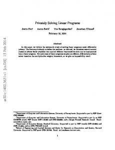
Figure 1 plots the numbers of pivoting steps in Phase I, Phase II, and Phase III, for the 168 LPCCs. We sorted the LPCCs by the number of variables n. As expected, larger programs tend to take more pivoting steps to solve. On the other hand, no phase dominated the computational cost in all cases. Detailed results are given in Tables 2–5.

LPCC pivoting count

5

10

4

10

# total pivots # pivots in Phase−I # pivots in Phase−II # pivots in Phase−III

# pivots

3

10

2

10

1

10

0

10

0

20

40

60

80

100

120

140

160

180

program index Figure 1: Pivoting counts of our pivoting algorithm using the MacMPEC-LPCC test set.

Figure 2 shows the performance profiles (Dolan and Moré, 2002; Dolan et al., 2006) of our pivoting algorithm and filter MPEC. In the left plot we use all 168 programs in the MacMPEC-LPCC test set. The plot indicates that our pivoting algorithm outperforms filter MPEC significantly. We note that filter MPEC sometimes takes orders of magnitude more pivoting steps than does our pivoting pivoting algorithm to verify the unbounded objectives. The reason may be that filter MPEC solves nonlinear MPECs and cannot take advantage of the possibility of unbounded linear rays. Therefore, in the right plot we remove the 30 unbounded problems. The results indicate that our pivoting algorithm still performs better.


20

excluding unbounded problems 1

0.9

0.9

0.8

0.8

0.7

0.7

% of problems

% of problems

full set 1

0.6 0.5 0.4 0.3

0.5 0.4 0.3

0.2

0.2

pivoting algorithm filter MPEC

0.1 0 0

0.6

2

4

6

log (# pivots / best # pivots) ≤ x

8

pivoting algorithm filter MPEC

0.1 10

2

0 0

2

4

6

log (# pivots / best # pivots) ≤ x

8

10

2

Figure 2: Performance profiles (log2 scale) using the MacMPEC-LPCC test set.

8 Conclusion We give a pivoting algorithm to solve linear programs with linear complementarity constraints. Our algorithm is based on the active set method for linear programming. It works under degeneracy and includes an anticycling scheme that can determine B-stationarity and avoid infinite loops. We also use an optimizationbased technique that consists of two phases to find an initial feasible vertex. Phase I is to find a linear feasible vertex, whereas Phase II is to resolve complementary violations. The experimental results indicate that our method is an appealing alternative to existing techniques.

Acknowledgments This work was supported by the Office of Advanced Scientific Computing Research, Office of Science, U.S. Department of Energy, under Contract DE-AC02-06CH11357. This work was also supported by NSF grant 0631622.

A

MacMPEC-LPCC Program Characteristics

Tables 2–5 list the following characteristic numbers of the 168 LPCCs in the MacMPEC-LPCC test set: the number of variables n, the number of constraints m, the number of equalities me , and the number of complementarity conditions p. The numbers of pivots of our pivoting algorithm and filter MPEC for each LPCC are also listed. Three error codes are used in these tables: “(d)” for the maximum degree of nonstrictness reached, “(i)” for the maximum number of iterations reached, and “(t)” for that trust region is too small.

References Anitescu, M. (2005). On using the elastic mode in nonlinear programming approaches to mathematical programs with complementarity constraints. SIAM J. Optim., 15:1203–1236.


21

Table 2: Results of the 168 programs in the MacMPEC-LPCC test set, Part I. Program bard1-lpcc bard1m-lpcc bard2-lpcc bard2m-lpcc bar-truss-3-lpcc bilevel1-lpcc bilevel1m-lpcc bilevel2-lpcc bilevel2m-lpcc bilevel3-lpcc bilin-lpcc bem-milanc30-s-lpcc dempe-lpcc design-cent-1-lpcc design-cent-21-lpcc design-cent-2-lpcc design-cent-31-lpcc design-cent-3-lpcc design-cent-4-lpcc desilva-lpcc df1-lpcc ex9.1.1-lpcc ex9.1.2-lpcc ex9.1.3-lpcc ex9.1.4-lpcc ex9.1.5-lpcc ex9.1.6-lpcc ex9.1.7-lpcc ex9.1.8-lpcc ex9.1.9-lpcc ex9.1.10-lpcc ex9.2.1-lpcc ex9.2.2-lpcc ex9.2.3-lpcc ex9.2.4-lpcc ex9.2.5-lpcc ex9.2.6-lpcc ex9.2.7-lpcc ex9.2.8-lpcc ex9.2.9-lpcc flp2-lpcc flp4-1-lpcc

n

m

me

p

5 6 12 12 35 10 8 16 16 10 8 3436 3 12 13 13 15 15 22 6 2 13 8 23 8 13 14 17 11 12 11 10 9 14 8 8 16 10 6 9 4 80

9 10 21 21 45 17 13 29 29 14 15 4901 3 15 19 19 15 15 33 8 2 18 13 35 13 20 21 26 17 18 17 15 14 23 12 11 22 15 9 14 5 90

1 1 5 5 28 2 2 4 4 6 0 1968 1 6 6 6 6 6 10 2 0 7 5 15 5 7 7 9 5 6 5 5 4 8 5 4 6 5 3 5 0 0

3 3 3 3 6 6 4 8 8 2 6 1464 1 3 3 3 3 3 8 2 1 5 2 6 2 5 6 6 3 5 3 4 3 4 2 3 6 4 2 3 2 30

# Pivots Pivoting Algor. Filter MPEC 6 8 5 8 7 8 7 9 10 15 8 8 6 12 12 20 12 20 5 3 8 165 8985 1517 2 3(i) 8 97 10 9 10 10 13 65(i) 9 63(i) 7 7 2 0 1 0 6 5 4 2 10 8 3 3 6 6 9 8 9 7 5 4 6 7 5 4 6 7 3 6 6 6 4 4 5 7 6 4 6 7 3 4 4 2 6 8 90 2829(t)


22

Table 3: Results of the 168 programs in the MacMPEC-LPCC test set, Part II. Program flp4-2-lpcc flp4-3-lpcc flp4-4-lpcc gauvin-lpcc gnash10m-lpcc gnash11m-lpcc gnash12m-lpcc gnash13m-lpcc gnash14m-lpcc gnash15m-lpcc gnash16m-lpcc gnash17m-lpcc gnash18m-lpcc gnash19m-lpcc hakonsen-lpcc hs044-i-lpcc incid-set1-8-lpcc incid-set1-16-lpcc incid-set1-32-lpcc incid-set1c-8-lpcc incid-set1c-16-lpcc incid-set1c-32-lpcc incid-set2-8-lpcc incid-set2-16-lpcc incid-set2-32-lpcc incid-set2c-8-lpcc incid-set2c-16-lpcc incid-set2c-32-lpcc jr1-lpcc jr2-lpcc kth1-lpcc kth2-lpcc kth3-lpcc liswet1-050-lpcc liswet1-100-lpcc liswet1-200-lpcc monteiroB-lpcc monteiro-lpcc nash1a-lpcc nash1b-lpcc nash1c-lpcc nash1d-lpcc

n

m

me

p

110 140 200 3 10 10 10 10 10 10 10 10 10 10 9 20 100 371 1517 100 371 1517 112 450 1857 112 450 1857 2 2 2 2 2 152 302 602 131 131 6 6 6 6

170 240 350 4 15 15 15 15 15 15 15 15 15 15 17 30 170 637 2559 177 652 2590 177 681 2767 184 696 2798 1 1 1 1 1 203 403 803 226 226 8 8 8 8

0 0 0 0 5 5 5 5 5 5 5 5 5 5 3 4 49 225 961 49 225 961 49 225 961 49 225 961 0 0 0 0 0 52 102 202 57 57 2 2 2 2

60 70 100 2 4 4 4 4 4 4 4 4 4 4 4 10 32 111 489 32 111 489 44 190 829 44 190 829 1 1 1 1 1 50 100 200 57 57 2 2 2 2

# Pivots Pivoting Algor. Filter MPEC 322 211 376 970(t) 1081 548 4 5 5 9 5 8 5 2 5 2 5 2 6 9 6 9 6 4 6 4 6 4 0 0 21 23 75 62 292 205 1492 935 88 78 435 237 1583 824 108 975 471 18038 2532 101792(t) 115 742 493 13251 2349 28910(t) 1 0 1 0 1 0 1 1 1 1 155 68(i) 309 140(i) 647 360(i) 218(d) 298 165(d) 136 2 5 4 10 6 12 4 11


23

Table 4: Results of the 168 programs in the MacMPEC-LPCC test set, Part III. Program nash1e-lpcc outrata31-lpcc outrata32-lpcc outrata33-lpcc outrata34-lpcc pack-comp1-8-lpcc pack-comp1-16-lpcc pack-comp1-32-lpcc pack-comp1c-8-lpcc pack-comp1c-16-lpcc pack-comp1c-32-lpcc pack-comp1p-8-lpcc pack-comp1p-16-lpcc pack-comp1p-32-lpcc pack-comp2-8-lpcc pack-comp2-16-lpcc pack-comp2-32-lpcc pack-comp2c-8-lpcc pack-comp2c-16-lpcc pack-comp2c-32-lpcc pack-comp2p-8-lpcc pack-comp2p-16-lpcc pack-comp2p-32-lpcc pack-rig1-8-lpcc pack-rig1-16-lpcc pack-rig1-32-lpcc pack-rig1c-8-lpcc pack-rig1c-16-lpcc pack-rig1c-32-lpcc pack-rig1p-8-lpcc pack-rig1p-16-lpcc pack-rig1p-32-lpcc pack-rig2-8-lpcc pack-rig2-16-lpcc pack-rig2-32-lpcc pack-rig2c-8-lpcc pack-rig2c-16-lpcc pack-rig2c-32-lpcc pack-rig2p-8-lpcc pack-rig2p-16-lpcc pack-rig2p-32-lpcc pack-rig3-8-lpcc

n

m

me

p

6 5 5 5 5 107 467 1955 107 467 1955 107 467 1955 107 467 1955 107 467 1955 107 467 1955 70 333 1433 70 333 1433 92 389 1711 75 326 1580 75 326 1580 91 369 1605 85

8 8 8 8 8 179 753 3101 186 768 3132 164 708 2948 179 753 3101 186 768 3132 164 708 2948 109 511 2171 116 526 2202 138 580 2571 120 510 2694 127 525 2725 139 565 2490 139

2 0 0 0 0 49 225 961 49 225 961 49 225 961 49 225 961 49 225 961 49 225 961 46 204 856 46 204 856 49 225 961 46 204 856 46 204 856 49 225 961 46

2 4 4 4 4 49 225 961 49 225 961 49 225 961 49 225 961 49 225 961 49 225 961 9 82 505 9 82 505 34 147 717 17 93 661 17 93 661 33 127 611 28

# Pivots Pivoting Algor. Filter MPEC 5 7 4 7 4 7 4 7 4 795(i) 1 27 1 143 1 624 1 27 1 141 1 655 84 83 339 347 1115 1049 1 25 1 161 1 262 1 25 1 161 1 251 86 93 294 293 1159 1003 47 32 250 185 781 186 39 26 253 174 781 186 83 72 386 240 2387 7443(t) 58 40 115 65 756 201 61 40 123 65 765 200 76 53 294 166 1536 577 65 42


24

Table 5: Results of the 168 programs in the MacMPEC-LPCC test set, Part IV. Program pack-rig3-16-lpcc pack-rig3-32-lpcc pack-rig3c-8-lpcc pack-rig3c-16-lpcc pack-rig3c-32-lpcc portfl-i-1-lpcc portfl-i-2-lpcc portfl-i-3-lpcc portfl-i-4-lpcc portfl-i-6-lpcc qpec1-lpcc qpec2-lpcc qpecgen-100-1-lpcc qpecgen-100-2-lpcc qpecgen-100-3-lpcc qpecgen-100-4-lpcc qpecgen-200-1-lpcc qpecgen-200-2-lpcc qpecgen-200-3-lpcc qpecgen-200-4-lpcc ralph1-lpcc ralph2-lpcc ralphmod-lpcc scale1-lpcc scale2-lpcc scale3-lpcc scale4-lpcc scale5-lpcc scholtes1-lpcc scholtes2-lpcc scholtes3-lpcc scholtes4-lpcc scholtes5-lpcc siouxfls-lpcc siouxfls1-lpcc sl1-lpcc stackelberg1-lpcc tap-09-lpcc tap-15-lpcc taxmcp-lpcc water-net-lpcc water-FL-lpcc

n

m

me

p

360 1490 85 360 1489 87 87 87 87 87 30 30 105 110 110 120 210 220 220 240 2 2 104 2 2 2 2 2 3 3 2 3 3 2403 2403 8 3 86 194 12 66 213

573 2342 146 588 2371 99 99 99 99 99 39 39 202 202 204 204 404 404 408 408 2 1 203 1 1 1 1 1 2 2 1 4 3 4703 4703 11 4 136 328 24 116 373

204 856 46 204 856 13 13 13 13 13 0 0 0 0 0 0 0 0 0 0 0 0 0 0 0 0 0 0 0 0 0 0 0 628 628 2 1 32 68 3 36 116

129 586 28 129 585 12 12 12 12 12 20 20 100 100 100 100 200 200 200 200 1 1 100 1 1 1 1 1 1 1 1 1 2 1748 1748 3 1 32 83 10 14 44

# Pivots Pivoting Algor. Filter MPEC 346 161 746 563 64 35 291 130 755 317 62 28 59 26 60 36 61 28 60 32 30 1 20 0 167 7689(i) 197 19385(i) 604 16161(i) 478 23855(i) 1047 24243(i) 1838 43704(i) 2825 41805 1022 27416 2 5 1 3 136 1515 0 2 0 2 0 3 0 3 0 3 3 2 4 2 1 1 4 6 1 3 10800 97578 11781 12225 6 10 2 0 76 118 159 274 22 134 37 11 135 43


25

Anitescu, M., Tseng, P., and Wright, S. J. (2007). Elastic-mode algorithms for mathematical programs with equilibrium constraints. Math. Program., 110:337–371. Audet, C., Hansen, P., Jaumard, B., and Savard, G. (1997). Links between linear bilevel and mixed 0-1 programming problems. J. Optim. Theory Appl., 93:273–300. Audet, C., Savard, S., and Zghal, W. (2007). New branch-and-cut algorithm for bilevel linear programming. J. Optim. Theory Appl., 134:353–370. Bartels, R. H. and Golub, G. H. (1969a). Algorithm 350: Simplex method procedure employing LU decomposition. Commun. of ACM, 12:275–281. Bartels, R. H. and Golub, G. H. (1969b). The simplex method of linear programming using LU decomposition. Commun. of ACM, 12:266–268. Benson, H., Sen, A., Shanno, D. F., and Vanderbei, R. V. D. (2006). Interior-point algorithms, penalty methods and equilibrium problems. Comput. Optim. Appl., 34(2):155–182. Campêlo, M. and Scheimberg, S. (2000). A note on a modified simplex approach for solving bilevel linear programming problems. European J. Oper. Res., 126:454–458. Chvátal, V. (1983). Linear Programming. W. H. Freeman & Company. Dolan, E. D. and Moré, J. J. (2002). Benchmarking optimization software with performance profiles. Math. Program. Ser. A, 91:201–213. Dolan, E. D., Moré, J. J., and Munson, T. S. (2006). Optimality measures for performance profiles. SIAM J. Optim., 16(3):891–909. Facchinei, F., Jiang, H., and Qi, L. (1999). A smoothing method for mathematical programs with equilibrium constraints. Math. Program., 85:107–134. Ferris, M. C., Fourer, R., and Gay, D. M. (1999). Expressing complementarity problems in an algebraic modeling language and communicating them to solvers. SIAM J. Optim., 9:991–1009. Fletcher, R. and Leyffer, S. (2004). Solving mathematical program with complementarity constraints as nonlinear programs. Optim. Methods Soft., 19(1):15–40. Fletcher, R., Leyffer, S., Ralph, D., and Scholtes, S. (2006). Local convergence of SQP methods for mathematical programs with equilibrium constraints. SIAM J. Optim., 17(1):259–286. Fletcher, R. and Matthews, S. P. J. (1984). Stable modification of explicit LU factors for simplex updates. Math. Program., 30(3):267–284. Fourer, R., Gay, D. M., and Kernighan, B. W. (2002). AMPL: A Modeling Language for Mathematical Programming. Duxbury Press, 2nd edition. Fukushima, M. and Tseng, P. (2002). An implementable active-set algorithm for computing a B-stationary point for a mathematical program with linear complementarity constraints. SIAM J. Optim., 12:724–739.

26


Gill, P. E., Murray, W., and Wright, M. H. (1990). Numerical Linear Algebra and Optimization. Addison Wesley Publishing Company. Goldfarb, D. and Reid, J. K. (1977). A practical steepest-edge simplex algorithm. Math. Program., 12:361– 371. Hansen, P., Jaumard, B., and Savard, G. (1992). New branch-and-bound rules for linear bilevel programming. SIAM J. Sci. Stat. Comput., 13(5):1194–1217. Hoheisel, T. and Kanzow, C. (2009). On the abadie and guignard constraint qualifications for mathematical programmes with vanishing constraints. Optimization, 58:431–448. Hu, J., Mitchell, J. E., Pang, J.-S., Bennet, K. P., and Kunapuli, G. (2008). On the global solution of linear programs with linear commplementarity constraints. SIAM J. Optim., 19:445–471. Hu, X. M. and Ralph, D. (2004). Convergence of a penality method for mathematical programming with complementarity constraints. J. Optim. Theory Appl., 123:365–390. Ibaraki, T. (1971). Complementary programming. Oper. Res., 19:1523–1529. Ibaraki, T. (1973). The use of cuts in complementary programming. Oper. Res., 21:353–359. Jiang, H. and Ralph, D. (2000). Smooth SQP methods for mathematical programs with nonlinear complementarity constraints. SIAM J. Optim., 10:779–808. Jiang, H. and Ralph, D. (2004). Extension of quasi-Newton methods to mathematical programs with complementarity constraints. Comput. Optim. Appl., 123:365–390. Leyffer, S. (2000). MacMPEC: AMPL www.mcs.anl.gov/˜leyffer/MacMPEC/.

collection

of

MPECs.

Web

page,

Leyffer, S. (2005). The penalty interior point method fails to converge. Optim. Methods Soft., 20:559–568. Leyffer, S. (2006). Complementarity constraints as nonlinear equations: Theory and numerical experience. In Dempe, S. and Kalashnikov, V., editors, Optimization with Multivalued Mappings, pages 169–208. Springer. Leyffer, S., Lopéz-Calva, G., and Nocedal, J. (2006). Interior methods for mathematical programs with complementarity constraints. SIAM J. Optim., 17(1):52–77. Leyffer, S. and Munson, T. S. (2007). A globally convergent filter method for MPECs. Preprint ANL/MCSP1457-0907, Argonne National Laboratory, Mathematics and Computer Science Division. ¨ Onal, H. (1993). A modified simplex approach for solving bilevel linear programming problems. European J. Oper. Res., 67:126–135. Pang, J.-S. and Fukushima, M. (1999). Complementarity constraint qualifications and simplified Bstationarity conditions for mathematical programs with equilibrium constraints. Comput. Optim. Appl., 13(1-3):111–136.


27

Scheel, H. and Scholtes, S. (2000). Mathematical program with complementarity constraints: Stationarity, optimality and sensitivity. Math. of Oper. Res., 25:1–22. Scholtes, S. (2001). Convergence properties of a regularization scheme for mathematical programs with complementarity constraints. SIAM J. Optim., 11:918–936. Stange, P., Griewank, A., and Bollhöfer, M. (2007). On the efficient update of rectangular LU-factorizations subject to low rank modifications. Electron. Trans. Numer. Anal., 26:161–177. Ye, J. J. (1999). Optimality conditions for optimization problems with complementarity constraints. SIAM J. Optim., 9(2):374–387. Ye, J. J. (2005). Necessary and sufficient optimality conditions for mathematical programs with equilibrium constraints. J. Math. Anal. Appl., 307:350–369.

The submitted manuscript has been created by the UChicago Argonne, LLC, Operator of Argonne National Laboratory (“Argonne”) under Contract No. DE-AC02-06CH11357 with the U.S. Department of Energy. This work was also supported by NSF grant 0631622. The U.S. Government retains for itself, and others acting on its behalf, a paid-up, nonexclusive, irrevocable worldwide license in said article to reproduce, prepare derivative works, distribute copies to the public, and perform publicly and display publicly, by or on behalf of the Government.