A Point-Matching Based Algorithm for 3D Surface ... - Semantic Scholar

A Point-Matching Based Algorithm for 3D Surface Alignment of Drug-Sized Molecules Daniel Baum and Hans-Christian Hege Zuse Institute Berlin (ZIB), Germany {baum,hege}@zib.de

Abstract. Molecular shapes play an important role in molecular interactions, e.g., between a protein and a ligand. The ‘outer’ shape of a molecule can be approximated by its solvent excluded surface (SES). In this article we present a new approach to molecular surface alignment which is capable of identifying partial similarities. The approach utilizes an iterative point matching scheme which is applied to the points representing the SES. Our algorithm belongs to the multi-start methods. We first generate a number of initial alignments that are locally optimized by an iterative surface point matching algorithm which tries to maximize the number of matched points while minimizing the distance between the matched points. The algorithm identifies similar surface regions given by the matched surface points. This makes it well suited for multiple alignment of molecular surfaces. The subalgorithm proposed for distributing points uniformly across a surface might be of general interest for the comparison of molecular surfaces.

1

Introduction

Molecular alignment is a widely used tool in pharmaceutical drug design. An alignment of molecular structures allows one to identify commonalities and differences among the molecular structures. Molecular alignment is thus a prerequisite for pharmacophore identification using Structure Activity Relationship (SAR) approaches. There exist many molecular alignment algorithms (see, e.g., [1]). Most of these algorithms consider the molecular ‘skeleton’. But there also exist approaches considering the ‘outer’ shape of the molecule, i.e., its molecular surface, e.g. [2–6]. Ritchie et al. [2] represent the molecular surface using spherical harmonics. While this approach is fast, it is restricted to globular molecules and is not suitable for partial surface matching. Goldman et al. [3] use quadratic shape descriptors. Single points on the surface together with the principal directions of curvature are used to align molecular surfaces. Cosgrove et al. [4] and Hofbauer [6] identify circular regions of approximately constant curvature into which they position points. They then apply clique detection on those points to align the molecular surfaces. Exner et al. [7] patchify the molecular surface into overlapping surface patches of similar properties employing fuzzy sets. This patchification is later used in a docking scheme [5] whereby they utilize geometric

hashing for the identification of complementary surface regions. Their approach could also be applied to the alignment of molecular surface regions. Molecular surfaces are also used in virtual screening for computing molecular descriptors, e.g. [8–10], which are used to screen data bases of potential drugs. Zauhar et al. [8] generate shape signatures from the molecular surface by propagating a random ray inside the molecular surface. Shape signatures represent a probability distribution of the measured distances within the molecular surface. This one-dimensional signature is used to compare the shapes of molecules. The approaches by Stiefl et al. [9] and Bender et al. [10] both use point distributions on the surfaces gained either directly from the molecular surface triangulation [10], or by approximating the molecular surface by points on a 3D uniform grid [9]. While in the first approach the points are not uniformly distributed across the molecular surface, the second approach positions the points not directly onto the surfaces and the point distribution is not transformation invariant. In this paper we introduce a new transformation invariant algorithm for distributing points uniformly across a molecular surface. We also propose a new molecular alignment algorithm based on uniformly distributed points on the surface.

2

Methods

In this section we describe the whole process of aligning two molecular surfaces based on a partial surface matching. At the core of the algorithm lies the representation of the solvent excluded surface (SES) by point sets. We have developed a new method to uniformly distribute a rather small number of points on a surface, given as a triangle mesh. The alignment procedure is a multi-start approach. We first generate a number of initial transformations of the surface point sets based on the identification of small common substructures of the molecular skeletons. To each initial transformation we apply an iterative point matching scheme [11–13] which was modified to meet the needs of surface alignment, including the handling of physico-chemical properties. 2.1

Surface Point Representation

To efficiently compute molecular surface alignments based on an iterative point matching scheme, we need to uniformly distribute points on the molecular surface. We compute high-resolution triangle meshes of the SES based on the algorithm of Totrov et al. [14], implemented in the molecular visualization and analysis tool amiraMol [15]. These triangle meshes are partitioned into equally sized surface patches using the graph-partitioning software library METIS [16], version 4.0. Into each surface patch we position a single point, representing the patch. Although this initial point positioning scheme works rather well, we need to relax the points to obtain a uniform point distribution. We have developed an approximate Voronoi diagram computation method on 2-manifold triangle

meshes based on the work of Deussen et al. [17], who use Voronoi diagrams to distribute points regularly in 2D. We also investigated the use of the remeshing approach proposed by Surazhsky et al. [18] which worked well for most surface meshes, but was unable to move close points in the presence of creases. Apart from this problem, the point distribution algorithm proposed here is much faster while not running into problems with creases. Initial Point Positioning. The input to our point distribution algorithm is a 2-manifold triangle mesh M. Let V = {v1 , . . . , vm } be the set of vertices of M and T = {t1 , . . . , tn } the set of triangles of M. For t ∈ T we denote by v(t, i) the i’th vertex of t, i ∈ {1, 2, 3}. Furthermore, we denote by x(v) the coordinates of vertex v ∈ V , by x(t) the coordinates of the barycenter of t ∈ T , by n(t) the normal vector of t, and by A(t) the area of t. Let N (v) denote the triangleneighbors of vertex v ∈ V , i.e. all triangles incident to v, and let N (t) denote the triangle-neighbors of triangle t ∈ T , i.e. the triangles that share a common edge with t. Let S(M) be a connected subpatch of M, i.e. for each two triangles t0 , t00 ∈ S(M), t0 6= t00 , there exists a k > 0 and a path (t0 , t1 , . . . , tk−1 , tk ) with t0 = t0 , tk = t00 , such that ti ∈ N (ti−1P ) ∩ S(M), ∀i = {1, . . . , k}. From the surface area A(T ) := t∈T A(t) and the specified point density ρ we compute the number of points N = A(T ) · ρ to be distributed on M. For partitioning M into N patches, we use the METIS method PartMeshDual, which needs as input the connectivity of the triangle mesh M, i.e. T and for each t ∈ T its vertices v(t, i), i ∈ {1, 2, 3}, and N . PartMeshDual first converts the mesh-graph into its dual by representing each triangle t by a node which is connected to the nodes representing the triangles ti ∈ N (t), i ∈ {1, 2, 3}. The PartMeshDual algorithm aims at minimizing the number of edge cuts of the dual graph while partitioning the dual graph into N equally sized connected nodepartitions. The node-partitioning SN is then assigned to the original mesh M, giving a triangle-partitioning M = i=1 Si (M), with Si (M) ∩ Sj (M) = ∅, ∀i 6= j. To obtain the initial point P positioning, for eachP subpatch Si (M) we compute its barycenter x(Si (M)) := and project it t∈Si (M) A(t)x(t)/ t∈Si (M) A(t) P P onto M using its normal vector n(Si (M)) := t∈Si (M) A(t)n(t)/ t∈Si (M) A(t) or the vector −n(Si (M)), depending on whether the barycenter is inside or outside of M, respectively. To do this efficiently, we use an octree in which we store all triangles of M. This allows us to quickly identify the triangles that are intersected by a ray from x(Si (M)) with direction n(Si (M)) or −n(Si (M)). We denote the points representing Si (M) by pi and its coordinates by x(pi ). Point Positioning Optimization. Let P := {p1 , . . . , pN } be the set of points distributed on M. Let t(p), p ∈ P, be the triangle in which x(p) lies. The optimization algorithm works as follows. First, compute the Voronoi diagram for X(P ) := {x(p1 ), . . . , x(pN )} on M. Second, compute the center of each Voronoi cell, Vi , and move x(pi ) to the center of Vi . We shortly recall the definition of the Voronoi diagram. For some space Ω, the Voronoi diagram of a finite set of points X := {x1 , . . . , xn } ⊆ Ω partitions Ω into Voronoi cells Vi , such that for

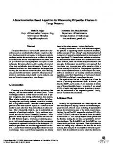
(a)

(b)

(c)

˜ (black). (c) Same as (b) Fig. 1. (a) Mesh M. (b) Mesh M (grey) and dual mesh M plus extended edges (dashed).

some distance metric dΩ it is true that dΩ (y, xi ) < dΩ (y, xj ), ∀y ∈ Vi , ∀i 6= j. In our case, where Ω = M, the appropriate distance metric would be the geodesic distance. However, the exact computation of the Voronoi diagram on a triangle mesh is very expensive to compute. We have therefore developed the following approximation method. Let E = {e1 , . . . , es } be the set of edges of M, and for some edge e ∈ E, let t(e, i), i ∈ {1, 2}, be the triangles adjacent to e. We now consider the ˜ of M, where each triangle t ∈ T is replaced by a vertex, v˜(t), dual mesh M with coordinates x(˜ v (t)) := x(t), and each edge e is replaced by its dual edge e˜ = (˜ v (t(e, 1)), v˜(t(e, 2))), connecting the dual vertices of t(e, 1) and t(e, 2). We ˜ by V˜ , and the set of edges of M ˜ by E. ˜ For each denote the set of vertices of M ˜ by edges from v˜(t) to the dual vertices of the triangles t ∈ T we now extend E adjacent to t’s vertices S v(t, i),Si ∈ {1, 2,S3}. This means, we define the extended ˜ 0 := dual edge set by E v (t), v˜(t0 )) (cf. Fig. 1). t∈T i∈{1,2,3} t0 ∈N (v(t,i)) (˜ Instead of computing the exact Voronoi diagram for X(P ) on M, we compute an approximation by collecting for each p ∈ P all triangles whose barycenters are closer to x(t(p)) than to any other x(t(p0 )), p0 ∈ P . The geodesic distances from x(t(p)) to the barycenters of the triangles of M are approximated by the ˜ 0 , denoted by d ˜ 0 (·, ·), length of the shortest paths on the extended dual edge set E E whereby we weight each edge by the Euclidean distance between the barycenters ˜0) connected by the edge. The shortest paths on the weighted graph G = (V˜ , E are computed using a modified version of Dijkstra’s algorithm starting from all v˜(t(p)) simultaneously. For each vertex v˜ ∈ V˜ , we not only store the current shortest distance, but also the point p ∈ P it is currently assigned to. SN The Voronoi cell approximation leads to a new partitioning M = i=1 Si0 (M), with Si0 (M) := {t | dE˜ 0 (˜ v (t(pi )), v˜(t)) < dE˜ 0 (˜ v (t(pj )), v˜(t)), ∀j 6= i}. With this partitioning we proceed as with the initial partitioning, resulting in new coordinates x(pi ) for all points pi ∈ P . We repeat this procedure until no points are moved anymore or until a maximum number of iterations has been performed. ˜ 0 ) instead of on The reason for computing the shortest paths on G = (V˜ , E ˜ ˜ G = (V , E) lies in the much better approximation of the geodesic distances than ˜ In order to produce good results, M needs to have a rather fine when using E. resolution. We have obtained good results for a point density of 20 points per 2 ˚ A for M (cf. Fig. 2).

(initial patches)

(after 10 iterations)

(initial patches)

(after 15 iterations)

Fig. 2. Patchification and point distribution on the SES of Tipranavir for different resolutions and at different times of iteration. Top row: 139 points with an approximate point distance of 2.0 ˚ A. Bottom row: 559 points with an approximate point distance of 1.0 ˚ A.

2.2

Surface Point Matching

Let P and Q be two surface point sets with corresponding coordinate sets X(P ) and X(Q) generated using the point distribution algorithm described in Sec. 2.1. We define a matching on P and Q as a bijection f : P 0 → Q0 , with P 0 ⊆ P and Q0 ⊆ Q. A matching f can be written as a set f ∗ of pairs from P × Q with (p, q) ∈ f ∗ ⇔ f (p) = q. The number of pairs |f ∗ | will be referred to as the size of f . We define the root mean square distance (rmsd) of the two point sets with respect to a matching f and a rigid body transformation T as sP 2 (p,q)∈f ∗ kx(p) − T (x(q))k rmsd(P, Q; f ; T ) := . (1) |f ∗ | We further define the matching score w.r.t. T as score(P, Q; f ; T ) :=

|f ∗ | · e−α·rmsd(P,Q;f ;T ) , min(|P |, |Q|)

(2)

with α ∈ R+ . The parameter α allows us to weight the importance of the rmsd. For a given transformation T we compute matchings of sizes 1 to min(|P |, |Q|) using a greedy strategy [12]. Set f0∗ = ∅, P0 = P , and Q0 = Q. From fi∗ we ∗ compute fi+1 by adding (p0 , q 0 ) ∈ Pi × Qi with d(p0 , q 0 )