A Probabilistic Tabu Search Algorithm for the Generalized Minimum Spanning Tree Problem Diptesh Ghosh P&QM Area, IIM Ahmedabad, Vastrapur, Ahmedabad 380015, India
[email protected] July 3, 2003 Abstract In this paper we present a probabilistic tabu search algorithm for the generalized minimum spanning tree problem. The basic idea behind the algorithm is to use preprocessing operations to arrive at a probability value for each vertex which roughly corresponds to its probability of being included in an optimal solution, and to use such probability values to shrink the size of the neighborhood of solutions to manageable proportions. We report results from computational experiments that demonstrate the superiority of this method over the generic tabu search method. Keywords: Probabilistic Tabu Search, Generalized Minimum Spanning Tree Problem, Latin Hypercube
1
Introduction
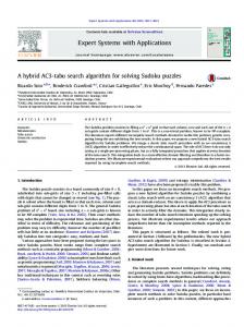
Consider a graph G = (V, E), in which the vertex set V is partitioned into m subsets (clusters), V1, V2, . . . , Vm, containing k1, k2, . . . , km vertices respectively. Assume that edges of the form (p, q), p, q ∈ Vi do not exist in E. The Generalized Minimum Spanning Tree Problem (GMSTP) is the problem of choosing one vertex from each of the subsets V1, V2, . . . , Vm, and connecting them through a minimum spanning tree, such that the cost of the tree is the minimum possible. Figure 1(a) shows a partitioning of the vertex set in a GMSTP instance, and Figure 1(b) shows a possible solution. The GMSTP is one of several generalized network design problems (see Feremans, Labb´e, and Laporte [3] for a review of generalized network design problems). It was first proposed in Myung, Lee, and Teha [8] and has been comprehensively reviewed in Feremans [5]. In the published literature, several alternate formulations for the GMSTP have been proposed in Feremans [5], Faigle, Kern, Pop, and Still [2], Myung, Lee, and Teha [8]. Myung Lee and Teha [8] proved that the problem is NP-Hard, even though the underlying minimum spanning tree problem is polynomial. Feremans [5] has experimented with exact algorithms, while Dror, Hauori, and Chaouachi [1], Myung, Lee, and Teha [8], and Pop, Kern, and Still [9] have proposed approximation algorithms and heuristics. 1
(a) Partitioning the vertex set
(b) A possible solution
Figure 1: The Generalized Minimum Spanning Tree Problem Dror, Hauori, and Chaouachi [1], Feremans, Labb´e, and Laporte [4], Ihler, Reich, and Widmayer [6] have dealt with problems closely related to the GMSTP. To the best of our knowledge, sophisticated metaheuristic techniques have not been applied to this problem, although Dror, Hauori, and Chaouachi [1] have proposed an elementary genetic algorithm, and Feremans [5] has mentioned an elementary tabu search technique with short term memory structures to obtain upper bounds to the GMSTP. In this paper, we propose a new tabu search algorithm for the GMSTP, and compare its performance against a generic tabu search algorithm on large randomly generated problem instances. Section 2 introduces our variant of tabu search and Section 3 reports our computational experiences with the algorithm. We conclude the paper with a few suggestions for future work in this area in Section 4.
2
The Tabu Search Approach
In this section we introduce our version of tabu search, after describing a generic tabu search algorithm, which we will use to benchmark out algorithm. In our implementations, we assume that k1 = K2 = · · · = km = k. A solution to the GMSTP instance with m clusters is a m-tuple defined on the alphabet 1, . . . , k. If the ith entry in a solution is j, then it means that the vertex labelled (i − 1) × k + j will be use in the tree representing that solution. The cost of the solution is the cost of the minimum cost tree spanning the vertices included in the solution. For example, let us consider an instance with 5 clusters, each having 4 vertices. The solution S = (4, 1, 2, 3, 2) to this instance represents the minimum cost tree spanning vertices 4, 5, 10, 15, and 18, and the cost of S is the cost of that tree. A neighbor of a solution is a solution that has exactly one entry different from the original solution. For example, the solution S1 = (4, 1, 3, 3, 2) is a neighbor of S. Given this solution representation and neighborhood structure, a generic tabu 2
search implementation would involve the following steps: Generic Tabu Search (GTS) Step 1 (Initialization): Define all solution elements as non-tabu. Choose an initial solution S, set BestSolution ← S, and set Iteration ← 1. Go to Step 1. Step 2 (Termination): If a pre-defined termination condition is satisfied, output BestSolution and exit. Else go to Step 3. Step 3 (Iteration): Consider all neighbors of S. All such neighbors for which a move to that neighbor requires the use of a solution element marked ‘tabu’ are tabu neighbors, while all others are ‘non-tabu’ neighbors. If the best tabu neighbor has a cost lower than the cost of BestSolution, go to Step 4, else replace S by the best non-tabu neighbor of S. Mark the solution elements participating in this move (i.e. the vertex that has left the solution, and the vertex that has entered the solution to form the neighbor) as tabu for the next TENURE moves. If this best non-tabu neighbor is better than BestSolution, replace BestSolution with this neighbor. Set Iteration ← Iteration + 1. Go to Step 2. Step 4 (Aspiration): Replace BestSolution and S with the tabu neighbor of S. Remove the tabu status for all solution elements. Set Iteration ← Iteration + 1. Go to Step 2. The main problem with such a tabu search algorithm is the size of the neighborhood, for each solution, there are km neighbors to evaluate. Thus GTS is able to execute only a few iterations within reasonable execution times. Our version of tabu search addresses this concern. The basic idea in our version is to look at only a subset of the neighborhood of each solution which has the maximum likelihood of containing the best tabu and non-tabu neighbors. We work under the belief that a large enough set of locally optimal solutions collectively contain predominantly those features that are present in globally optimal solutions and rarely contain features that are absent in globally optimal solutions. Under this belief, we start our version by generating a pre-determined number s of initial solutions using an extension to the Latin hypercube (s is typically a multiple of k; see McKay, Conover, and Beckman [7] for details). We run steepest descent local search procedures starting with each of these solutions and arrive at locally optimal solutions close to each of them. We then define a probability of each vertex vi ∈ V appearing in an optimal solution in the following manner. Let the vertex vi appear in ni of the s local optima obtained above. Also, let vmax be the vertex belonging to the same cluster, and which is observed in the maximum number of local optima (nmax ). Then the probability associated with vi is (ni + α)/(nmax + α) where α is a pre-determined constant. Once these probabilities are defined, we look at
3
neighbors of a solution based on the probability of the corresponding moves leading towards optimal solutions. For example, if the probability associated with vertex vi is pi, and that associated with another vertex vj in the same cluster is pj, then a move that removes the vertex vi from the solution and includes vj is executed with a probability of (1 − pi)pj. The parameter α determines the severity that we assume in not looking at moves that either exclude a vertex commonly observed in the set of local optima, or include a vertex that is not common in the set of local optima. Our version of tabu search is formalized below: Probabilistic Tabu Search (PTS) Step 0 (Generating Probabilities): Generate a set of s solutions S = {S1, S2, . . . , Ss} using an extension to the Latin hypercube. For each Si ∈ S, apply a steepest descent local search method to obtain a local optimum LSi. For each vi ∈ V, the vertex set, compute the associated probability pi. Go to Step 1. Step 1 (Initialization): Define all solution elements as non-tabu. Choose an initial solution S, set BestSolution ← S, and set Iteration ← 1. Go to Step 1. Step 2 (Termination): If a pre-defined termination condition is satisfied, output BestSolution and exit. Else go to Step 3. Step 3 (Iteration): Consider each neighbor N of S with a probability of (1 − pi)pj where vi = S \ N and vj = N \ S. If vi or vj is marked ‘tabu’ then N is a tabu neighbor, otherwise it is a ‘non-tabu’ neighbor. If the best tabu neighbor considered has a cost lower than the cost of BestSolution, go to Step 4, else replace S by the best non-tabu neighbor considered. Mark the solution elements participating in this move (i.e. the vertex that has left the solution, and the vertex that has entered the solution to form the neighbor) as tabu for the next TENURE moves. If this best non-tabu neighbor is better than BestSolution, replace BestSolution with this neighbor. Set Iteration ← Iteration + 1. Go to Step 2. Step 4 (Aspiration): Replace BestSolution and S with the tabu neighbor of S. Remove the tabu status for all solution elements. Set Iteration ← Iteration + 1. Go to Step 2.
3
Computational Experience
We implemented both GTS and PTS in C and compiled them using the generic cc compiler under the Linux operating system. Since the problem instances generated were too large to solve to optimality we tested the performance of PTS using the performance of GTS as a benchmark. We generated eleven sets of test problems. Each set consisted of ten randomly generated instances. Each 4
d1
m=4
d2
n=7
Figure 2: Explaining variables used in instance generation of the instances were Euclidean, i.e. the distance matrices obeyed the triangle inequality. The vertices in each cluster are scattered randomly over a square of side d1 units. The clusters themselves are arranged in a rectangular grid such that the inter-cluster distance is d2 units. There are n clusters in each row of the grid, and there are m such columns. A typical arrangement of clusters is shown in Figure 2. If m and n are equal, it represents an instance defined on a square, but if they are quite different, the instance is defined on a much narrower rectangular area. Thus m and n together control the underlying shape of the instance. If d1 and d2 are equal, then the clusters are arranged one against the other. If d2 is significantly larger than d1, then the instance generated models a situation where the vertex clusters are widely separated. This kind of situation is very typical in conventional distribution networks. If d1 is larger than d2, then the clusters overlap. This happens mostly when we consider the problem of interconnecting computer networks that share the same geographical region. Details of the eleven problem sets generated are shown in Table 1. After a set of preliminary experiments, we set TENURE to 10 iterations for both GTS and PTS algorithms. The value of α was set equal to the value of k. We observed that setting s in PTS to a relatively high value resulted in a better selection of the probability value associated with each vertex. However, a high value of s required that more time was spent in the construction of the locally optimal solutions for generating the probabilities (Step 0 in PTS) which in turn led to less time being available for the iterative tabu search procedure. Our preliminary experiments suggested that setting s to 2k yielded the best results. Each instance was allowed an execution time of 300 CPU seconds for both GTS and PTS on a Pentium machine operating at 450 MHz. The cost of the best solution generated by the algorithms at the end of the stipulated time was chosen as a measure of the performance of the algorithm. Since we use the GTS solution as a benchmark, we report the ratio of the cost of the PTS solution and 5
Table 1: The problem sets used in computational experiments
Set Set Set Set Set Set Set Set Set Set Set Set
1 2 3 4 5 6 7 8 9 10 11
m 15 15 15 25 45 15 25 45 15 25 45
Characteristics n p d1 d2 15 3 1.0 1.0 15 4 1.0 1.0 15 5 1.0 1.0 9 4 1.0 1.0 5 4 1.0 1.0 15 4 1.0 0.5 9 4 1.0 0.5 5 4 1.0 0.5 15 4 0.5 1.0 9 4 0.5 1.0 5 4 0.5 1.0
the cost of the GTS solution as our performance parameter. The value reported is the average of the ratios obtained for all ten instances in the set. The results we obtained are presented in Table 2. Table 2: Results from computational experiments
Set Set Set Set Set Set Set Set Set Set Set Set
1 2 3 4 5 6 7 8 9 10 11
Solution cost ratio Maximum Minimum Average 1.003 0.995 0.999 1.001 0.974 0.990 1.128 1.008 1.052 0.997 0.978 0.987 0.996 0.958 0.984 0.996 0.979 0.992 1.006 0.979 0.994 0.995 0.983 0.990 1.016 0.978 0.997 1.017 0.980 0.991 1.017 0.939 0.991
In all but one set (Set 3) the average ratio of solution costs is less than unity, which means that associating probability values to vertices and exploring neighborhoods based on these probabilities improves the chance of tabu search reaching better solutions within the same time than conventional tabu search. However, in several cases, the maximum value of the ratio is more than unity. Thus in some cases at least, the probability values prevent tabu search from reaching good local optima. 6
Our experiments are inconclusive about the effect of the cardinality of the vertex set on the performance of PTS. This is because no clear trend was observed while comparing sets 1, 2, and 3. However the effect of the shape of the instance on the performance of PTS was clearer. On comparing sets 2, 4, and 5; 6, 7, and 8; and 9, 10 and 11; it was clearer that PTS outperforms GTS most clearly when m and n differed widely. Observing sets 2, 6, and 9; 4, 7, and 10; and 5, 8, and 11; we see that PTS outperforms GTS most comprehensively when d1 = d2. It is least effective when d1 < d2. Therefore we can conclude that the probabilistic tabu search procedure we define here will be more effective when the distance between clusters is comparable or is large compared to area occupied by the clusters.
4
Directions for Future Work
In this paper, we develop a probabilistic tabu search algorithm for the Generalized Minimum Spanning Tree Problem. In this approach, a pre-defined number of starting solutions are chosen from widely separated regions in the sample space, and used in local search procedures to obtain a set of locally optimal solutions. These locally optimal solutions are then examined to provide an idea about the probability of each vertex being included in an optimal solution to the instance. Using these ideas, the neighborhood of each solution is searched in a probabilistic manner, such that the moves excluding vertices that have a high probability of being in an optimal solution or of including vertices that have a low probability of being in an optimal solution are discouraged. Our computational experience shows us that this probabilistic tabu search method outperforms generic tabu search most of the time. Two extensions to this probabilistic tabu search method are quite natural. First, we can consider the effect of including long term memory management and then observe the combined effect of such memory management and probabilistic neighborhood search on the solution quality. Second, we can also consider an adaptive probabilistic tabu search process, in which we do not choose the initial solutions using the extension to the Latin hypercube, but use high quality locally optimal solutions reached by the tabu search process itself to guide the search in future iterations. Our preliminary experiments with the adaptive algorithm are encouraging. Finally, we can consider such probabilistic tabu search methods to other problems, especially the less-researched generalized network design problems.
References [1] Dror, M., Haouari, M., and Chaouachi, J. (2000), Generalized spanning trees, European Journal of Operational Research 120, 583–592. [2] Faigle, U., Kern, W., Pop, P.C. and Still, G. (2000), The generalized minimum spanning tree problem, Working Paper, Department of Operations Re-
7
search and Mathematical Programming, University of Twente, The Netherlands. [3] Feremans, C., Labb´e, M. and Laporte, G. (2003), Generalized network design problems, European Journal of Operational Research 148, 1–13. [4] Feremans, C., Labb´e, M. and Laporte, G. (2001), On generalized minimum spanning trees, European Journal of Operational Research 134, 457–458. [5] Feremans, C. (2001), Generalized Spanning Trees and Extensions, Ph.D. Dissertation, Universit´e Libre de Bruxelles. [6] Ihler, E., Reich, G. and Widmayer, P. (1999), Class Steiner trees and VLSI design, Discrete Applied Mathematics 90, 173–194. [7] McKay, M.D., Conover, W.J. and Beckman, R.J. (1979), A comparison of three methods for selecting values of input variables in the analysis of output from a computer code, Technometrics 21, 239–245. [8] Myung, Y.S., Lee, C.H. and Teha, D.W. (1995), On the generalized minimum spanning tree problem, Networks 26, 231–241. [9] Pop, P.C., Kern, W. and Still, G.J. (2001), An approximation algorithm for the generalized minimum spanning tree problem with bounded cluster size, Working Paper, Department of Operations Research and Mathematical Programming, University of Twente, The Netherlands.
8