Bioinformatics Advance Access published February 26, 2009
A Robust Peak Detection Method for RNA Structure Inference by High-throughput Contact Mapping Jinkyu Kim 1 , Seunghak Yu 1 , Byonghyo Shim 2 , Hanjoo Kim 1 , Hyeyoung Min 3 , Eui-Young Chung 4 , Rhiju Das 5 , and Sungroh Yoon 1∗ School of Electrical Engineering, Korea University, Seoul 136-713, Korea Department of Computer Science, Korea University, Seoul 136-713, Korea 3 Department of Statistics, Stanford University, Stanford, CA 94305, USA 4 Department of Electrical and Electronic Engineering, Yonsei University, Seoul 120-749, Korea 5 Departments of Biochemistry and Physics, Stanford University, Stanford, CA 94305, USA 1 2
Associate Editor: Prof. Anna Tramontano
ABSTRACT Motivation: For high-throughput prediction of the helical arrangements of large RNA molecules, an innovative method termed multiplexed hydroxyl radical (·OH) cleavage analysis (MOHCA) has been proposed (Das et al., 2008). A key step in this promising technique is to detect peaks accurately from noisy radioactivity profiles. Since manual peak finding is laborious and prone to error, an automated peak detection method to improve the accuracy and throughput of MOHCA is required. Existing methods were not applicable to MOHCA due to their high false positive rates. Results: We developed a two-step computational method that can detect peaks from MOHCA profiles in a robust manner. The first step exploits an ensemble of linear and nonlinear signal processing techniques to find true peak candidates. In the second step, a binary classifier trained with the characteristics of true and false peaks is used to eliminate false peaks out of the peak candidates. We tested the proposed approach with 2002 MOHCA cleavage profiles and obtained the median recall, precision, and F-measure values of 0.917, 0.750, and 0.830, respectively. Compared with the alternatives considered, the proposed method was able to handle false peaks substantially better, thus resulting in 51.0–71.8% higher median values of precision and F-measure. Availability: The software and supplemental data are available at http://dna.korea.ac.kr/pub/mohca. Contact:
[email protected]
1
INTRODUCTION
Determining ribonucleic acid (RNA) structures is critical for biological research. Despite advances in related technology and a large effort to uncover RNA structures, progress has been slow due to the challenges in processing thousands of RNA samples in a highthroughput manner. Among many techniques developed to constrain RNA structure models, hydroxyl radical cleavage patterns have been used to acquire accurate residue-residue distance constraints. In spite of its accuracy, it is still unwieldy to investigate the structure of a large RNA molecule using the cleavage mapping method, because ∗ to
whom correspondence should be addressed
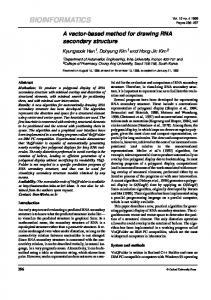
it is laborious and expensive to tether cleavage agents to each residue in a large RNA molecule. For high-throughput prediction of large RNA molecules, Das et al. (2008) proposed an innovative method termed multiplexed hydroxyl radical (·OH) cleavage analysis (MOHCA). This method randomly incorporates radical cleavage agents followed by twodimensional gel electrophoresis to detect pairs of contacting residues within a structured RNA molecule. The information on residue-residue interactions is then translated into constraints for modeling tertiary structure with the fragment assembly of RNA (FARNA) method (Das and Baker, 2007). A flowchart of MOHCA is shown in Figure 1(a). To randomly incorporate cleavage agents into RNA, Das et al. (2008) first performed in vitro transcription of the RNA in the presence of a modified nucleotide triphosphate (one type at a time) at a frequency of one modification per RNA. The modified nucleotide contains a 2’-amino group for attachment of the cleavage agent (an Fe-EDTA chelate) and a phosphorothioate group for specific cleavage to locate the position of the cleavage agent. Then the RNA is radio-labeled and a cleavage agent is tethered to the modified nucleotide. The pool of RNA molecules is gel purified and folded to the desired state, and radical generation is initiated by reducing Fe(III) to Fe(II). The cleavage products are separated by polyacrylamide gel electrophoresis to identify the cleavage position. The cleaved RNA molecules in the gel are then treated with iodine to induce backbone scission at the phosphorothioate and separated in the orthogonal dimension to identify the position of the responsible cleavage agent. Figure 1(b) shows the image of a 2-dimensional MOHCA gel, where each vertical strip represents a cleavage profile generated by a different source residue. The cleavage profile due to a radical source at A115 (Adenosine at 115) for the gel is shown in Figure 1(c) with four replicates independently prepared. In each cleavage profile, the peak location corresponds to the location of the nucleotide hit by the radical source at A115. Since the sequence of the sample RNA is already known, one can deduce the type of nucleotide at the position indicated by the peak. Secondary structure of the molecule (Figure 1(d)) is then generated with the constraints inferred from the gel, and its tertiary structure is determined by FARNA (Figure 1(e)). A key step in the entire MOHCA method is therefore to accurately detect the peak location in each cleavage profile. The peak locations
© The Author (2009). Published by Oxford University Press. All rights reserved. For Permissions, please email:
[email protected]
1
Kim et al.
Transcription reaction
Gel separation in the first direction
Radio-labeling I2 cleavage Coupling of 2'-amino-2'deoxy nucleotide-modified RNAs to ITCB-EDTA and Fe(III) loading
Gel separation orthogonal to the initial direction
Gel purification
Semi-automated analysis of MOHCA gels
25 Å
. OH cleavage Quantitative analysis of MOHCA cleavage patterns
(a)
(b)
(c)
(d)
(e)
120
130
140
150
160
170
A123
A122 A115
A114
A113
260 250 240 230 220 210 200 190 180
Fig. 1. Inferring RNA structure by MOHCA (Das et al., 2008). (a) Flowchart of MOHCA. (b) A sample MOHCA gel image with cleavage agents tethered to adenosine. (c) The cleavage profile (red) due to Fe(II) tethered at A115 for the gel in (b) and four replicates. (d) The native secondary structure for the P4-P6 domain of the Tetrahymena ribozyme with the constraints inferred from the gel in (b) overlaid. Cleavage agents (filled circle) are connected to representative cleaved residue (open circles). (e) A structural model using FARNA constrained by MOHCA with rainbow coloring from blue (5’) to red (3’).
Fig. 2. Five cleavage profiles from an actual MOHCA experiment. In each profile, the x and y axes correspond to the position of ·OH cleavage and intensity, respectively. Each potential hit judged by eyes is marked with a solid dot. Any hits that appeared to be gel smudges, nucleases, or spectator hits (i.e. present in other profiles) are marked with open circles. Each profile shares a background cleavage pattern due to the occasional presence of extra spectator sources on the RNA. This background often has apparent peaks, but these are not correct hits. The dotted lines mark where RNA products corresponding to different cleaved residues would run on the gel.
in each profile correspond to the position of the nucleotides that are interacting with a radical source, and the peak detection performance will eventually affect the quality of structure inference to a great extent. Consequently, in the original MOHCA study, the peak location in each cleavage profile was selected and verified manually, which limited the overall throughput of MOHCA. Due to gel smudges, nucleases, heterogeneous remnants from cleavage events, and the additive noise from observation instruments, the cleavage profile is usually very noisy and contains many false peaks. This makes it challenging to automate the peak detection process. For example, Figure 2 shows five cleavage profiles from an actual MOHCA experiment. The top profile indicates that the resulting cleavages (as shown by peaks) occur by the radical source at position 113, and the hit nucleotide is the residue at position 207. Small peaks at position 199, 172, and 155 are considered as false positives. The true “hit” is indicated by a black dot and the false hits by white dots.
2
The conventional techniques we tested tend to erroneously filter out important signals while preserving false peaks. For instance, continuous wavelet transform-based pattern matching (CWT) (Du et al., 2006) and the PROcess package included in Bioconductor (Gentleman et al., 2004), which were developed mainly for analyzing mass spectrometry data, show rather unsatisfactory detection performance on MOHCA profiles. In addition, popular signal processing techniques such as low-pass filtering (LPF; Oppenheim and Schafer, 1989) followed by zerocrossing detection in the derivative produce too many false peaks. Using these existing methods typically results in high misdetection rates and is of little use for MOHCA peak detection. We propose a new computational method for accurately detecting peaks from many MOHCA profiles in a high-throughput manner. As outlined in Figure 3, the proposed approach consists of two major steps called intra-profile peak detection and inter-profile peak analysis. The first intra-profile step considers individual cleavage profiles and collects peak candidates from each profile using an ensemble of sophisticated signal processing techniques. The focus of this step is to reduce false negative rates or to discover as many true peaks as possible. It is thus possible that the peak collection may contain false positives. The second inter-profile step is to eliminate such false peaks by considering multiple cleavage profiles simultaneously. To distinguish true and false peaks, we use an SVM-based binary classifier (Bishop, 2007) trained with labeled peaks with respect to features extracted from both spatial and Fourier domains. We next describe our results in detecting peaks by the proposed method from cleavage profiles collected from actual MOHCA experiments.
2
RESULT AND DISCUSSION
We tested the proposed peak detection method with the profiles obtained from 2002 gels used in 79 batches of MOHCA experiments. These gels covered all possible radical source attachment points, both 5’ and 3’ labeled samples, and different RNA solution conditions. Our technique was then compared with
A Robust Peak Detection Method
1.0 Profiles with labeled peaks
Feature extraction
Classifier (training phase)
Profiles
High-intensity noise rejection
Feature extraction
Nonlinear peak amplification
Classifier (prediction phase)
Derivative & smoothing operation
Peak labels
0.8
0.6
Intra-profile peak detection
Potential peaks
0.4
Inter-profile peak analysis
0.2
0.0
Fig. 3. Overview of the proposed approach.
P
Pi
C1
C5
C12
L21
L101 L1001
L21
L101 L1001
L21
L101 L1001
(a) Recall Detected peaks
True peaks FN
TP
1.0
FP
0.8
Fig. 4. We defined TP, FP, and FN peaks as detected true peaks, falsely detected peaks, and undetected true peaks, respectively.
several alternatives including CWT (Du et al., 2006) and LPFbased methods (Oppenheim and Schafer, 1989) in terms of three widely-used performance measures — recall, precision, and Fmeasure (Witten and Frank, 2005; Manning and Sch¨utze, 1999). The execution time and space requirement of all the techniques tested were negligible and not compared. CWT was chosen because it is one of the most advanced algorithms in terms of robustness, efficiency and ease of use. Although CWT was originally developed for mass spectrometry data, it was able to detect peaks in MOHCA profiles to some extent. The LPF-based technique was included due to its popularity and wide applicability in the signal processing area. Besides, we tested the PROcess package included in Bioconductor (Gentleman et al., 2004) but failed to make it detect any meaningful peaks, and no further result comparison were made for PROcess. There also exist deconvolution-based peak detection techniques for gas chromatography data (e.g. Viv´o-Truyols et al., 2005), but they were not included in comparison since we found that MOHCA peaks do not fit well the peak model used in these methods. Figures 5–9 summarize our results; more details of the profiles used and the full statistics obtained are available in the supplement. For notational convenience, we refer to the tested methods by the short labels defined in the caption of Figure 5. Of note is that a partial implementation of our approach, namely the first intra-profile step alone, was included in comparison. We wanted to assess how well this part performs by itself and how much performance gain the second inter-profile step adds thereafter. In order to compute precision, recall, and F-measure, we defined true positive (TP), false positive (FP), and false negative (FN) peaks as illustrated in Figure 4. Note that true negatives cannot be defined P in our context. Recall is given by F NT+T and indicates the fraction P of detected true peaks out of all true peaks. The maximum value of recall is 1, and recall decreases as the number of undetected true peaks (i.e. false negatives) increases. Precision is defined as TP and represents the portion of true peaks out of all detected T P +F P
0.6
0.4
0.2
0.0 P
Pi
C1
C5
C12
(b) Precision 1.0
0.8
0.6
0.4
0.2
0.0 P
Pi
C1
C5
C12
(c) F-measure (α = 0.25) Fig. 5. (Updated) Performance comparison: recall, precision, and Fmeasure values measured over 2002 MOHCA profiles. The line in the middle of a box indicates the median position, and the upper and lower boundaries represent the locations of the 75th and 25th percentiles, respectively. Symbol + indicates an outlier. The peak detection methods used and their labels are as follows: P: proposed method, Pi: proposed method (intra-profile step only), C1: CWT (SNR > 1), C5: CWT (SNR > 5), C12: CWT (SNR > 12), L21: 21-tap LPF, L101: 101-tap LPF, L1001: 1001-tap LPF. The normalized passband frequency of all LPFs is 0.01. Refer to the supplement for additional results.
3
Kim et al.
1.0
: Manual :P : C5 : L21
A140
0.9 0.8 0.7
Intensity
A136
A133
F-measure
A139
0.6 0.5 0.4 0.3
A125
0.2 A123 100
0.1 200
400 500 300 Position of OH cleavage
.
600
700
Fig. 6. (Updated) Peaks detected from a typical profile set by the different techniques tested (profile set used: mk84-Abomb-5prime-Unfolded). The proposed method detects much fewer false positive peaks than the alternatives.
peaks. A perfect detector would have precision of 1, but precision is lowered if false peaks are detected. F-measure can combine recall and precision into a single performance measure and is defined 1 as α/Precision+(1−α)/ Recall , where α is a parameter determining the weighting of precision and recall. The F-measure of a perfect peak detector would be 1. Figure 5 compares the proposed method with the alternatives with respect to the three comparison criteria. As far as recall is concerned, all the techniques tested resulted in high values, suggesting that few true peaks went undetected by using any of these methods. However, the precision of the proposed method was significantly higher than that of the others. This indicates that the proposed technique would typically detect much fewer false peaks (see Figure 6 for an example). Furthermore, the F-measure of the proposed method was much higher due to its higher precision. Figure 5 also reveals how the proposed technique achieves its performance advantage over the alternatives. The first intra-profile step seeks to minimize the number of false negatives (or undetected true peaks) to maintain high recall. The second step then prunes out most false peaks detected by the first step, for achieving high precision. Taken together, the proposed technique outperformed the competing methods by a large margin: The median precision and F-measure (α = 0.25) of our approach were higher by 64.0–71.5% and 51.0–71.8%, respectively. We further investigated how F-measure changes as varying α from 0 to 1. Given that F-measure is equal to recall when α = 0 and gradually becomes precision as α increases to 1, this test would reveal the relative performance of the compared techniques over all possible combinations of weights on precision and recall. As plotted in Figure 7, it is evident that the proposed technique consistently produced the highest level of F-measure for most α values. The performance of Pi and the LPF-based methods was slightly better only around α = 0. Figure 7 also indicates that using only the first half (i.e. label Pi) of our approach was sufficient to achieve higher F-measure than that the alternatives could provide. The full
4
0.0
0.1 P
0.2 Pi
0.3 C1
0.4 C5
0.5 0.6 alpha C12
0.7 L21
0.8 L101
0.9
1.0
L1001
Fig. 7. (Updated) F-measure comparison as α varies from 0 to 1. Each line corresponds to the average F-measure value of a certain technique calculated over 79 profile sets, and each vertical bar centered at the curve represents the standard error range around the average.
implementation of our approach (i.e. label P) showed even better F-measure leveraged by the second inter-profile step, only with a negligible performance loss near α = 0. One of recall and precision can be traded-off for boosting the other, and suboptimal detectors would have near perfect recall but very poor precision, or vice versa (Manning and Sch¨utze, 1999). To see how this trade-off occurs, we plotted in Figure 8(a) the twodimensional distribution of the precision and recall measured over all the 2002 profiles. For clarity in presentation, only the mean and standard deviation of each distribution are presented. As indicated in the figure, the proposed technique maintained balanced precision and recall over all the profile sets whereas the other methods skewed more towards high recall. In addition, the average precision of the proposed method was significantly higher, although the standard deviation values of some alternatives were smaller. In order to compare the baseline performance and robustness to noise, we selected 494 “noisy” profiles out of the entire 2002 profiles and measured the precision and recall therein. The true peaks appearing in these profiles were more difficult to distinguish from false peaks, according to our manual assessment described in Section 4.4. As shown in Figure 8(b), the impact of noise on precision and recall was marginal for all the methods tested. However, the performance of the proposed technique remained superior to that of the alternatives, and the precision-recall balance was also maintained well. Besides the three performance measures, we also compared the competing methods using the constraint maps of radical sources and cleavage sites. If two maps of constraints look similar, that will strongly suggest that the final RNA models predicted by FARNA or other tertiary structure predictors will also look similar. Figure 9 shows two sets of such maps, where the dots in each map correspond to the peak location predicted from the techniques in comparison. The circles in the maps indicate the locations of manually picked
A Robust Peak Detection Method
1.0
P
0.9
Pi
0.8
Manual
P
Pi
800
800
800
C1
600
600
600
C5
400
400
400
C7
200
200
Precision
0.7 0.6
L21
0.5
L101
0.4
L1001
120 140 160 180 200 220
200 120 140 160 180 200 220
C1
120 140 160 180 200 220
C5
C12
800
800
800
600
600
600
400
400
400
200
200
0.3 0.2 0.1 0.0 0.0 0.1 0.2 0.3 0.4 0.5 0.6 0.7 0.8 0.9 1 Recall
(a) Over the entire 2002 profiles 1.0
P
0.9
Pi
0.8
C1
200
120 140 160 180 200 220
120 140 160 180 200 220
L21
L101
120 140 160 180 200 220
L1001
800
800
800
600
600
600
400
400
400
200
200 120 140 160 180 200 220
200 120 140 160 180 200 220
120 140 160 180 200 220
(a) rd139b-Abomb-5prime-2MNaCl
C5
Manual
0.7
P
Pi
Precision
C7 0.6
L21
600
600
600
0.5
L101
400
400
400
0.4
L1001 200
200
200
0.3
120 140 160 180 200 220
120 140 160 180 200 220
120 140 160 180 200 220
0.2
C1
C5
C12
0.1
600
600
600
0.0
400
400
400
200
200
200
0.0 0.1 0.2 0.3 0.4 0.5 0.6 0.7 0.8 0.9 1 Recall
(b) Over 494 noisy profiles (selected from the entire profiles) Fig. 8. (Updated) Comparison of precision-recall distribution. Points of different shapes indicate the locations of the average precision and recall values of different detectors. Each two-dimensional error bar centered at a point represents the range set by the standard deviation around the average. More details of the 494 noisy profiles are available in the supplementary material. Table 1. The average MSE value of the constraint maps derived from each detection method over the 2002 profiles (all values normalized to P). Method
†
P
Pi
C1
C5
C12
L21
L101
L1001
1.00†
2.82
16.5
7.46
3.95
14.0
14.0
10.0
The original (unnormalized) value is 2.3744 × 10⁻⁵
peaks. As is evident in Figure 9, the map derived from the proposed method matches the manual map most closely. For more quantitative comparison, we also calculated the mean squared error (MSE; Kay, 1993) of every map with respect to the corresponding manual map. The average MSE value calculated for each method over the entire 2002 profiles is listed in Table 1; more details of computing MSE are explained in Section 4.4. It is clear that our technique can provide a constraint map that matches the manual map most closely.
120 140 160 180 200 220
120 140 160 180 200 220
120 140 160 180 200 220
L21
L101
L1001
600
600
600
400
400
400
200
200
200
120 140 160 180 200 220
120 140 160 180 200 220
120 140 160 180 200 220
(b) rd148c-thirdround-p4p6-CBOMB-5prime-unfolded-MKtop Fig. 9. Comparing maps of radical sources and cleavage sites. The x and y axes represent the locations of radical sources and cleavage sites, respectively, in an RNA sequence. A dot indicates the location of a predicted peak either manually (labeled ‘Manual’) or computationally (labeled ‘P’, ‘C5’, ‘L21’, etc.). The location of a manually picked peak (i.e. a dot in the ‘Manual’ map) is marked by a circle in the maps derived from the computational methods.
3 CONCLUSION We have developed a computational means to detect peaks appearing in the cleavage profile curves of the MOHCA method. The proposed approach combines signal processing techniques with supervised learning in order to maintain high true positive rates while suppressing detection of false peaks. Sensitivity and specificity analysis was performed using 2002 profiles collected from 79 batches of MOHCA experiments. The median recall, precision and F-measure (α = 0.25) values achieved were 0.917, 0.750 and 0.830, respectively, outperforming the alternatives
5
Kim et al.
tested by a large margin, especially in terms of precision and F-measure. These results suggest that our approach can be a very effective tool for enhancing the throughput and accuracy of MOHCA by automating its most time-consuming part, thereby making high-throughput prediction of RNA structures by MOHCA more attractive. Furthermore, it would be possible to apply our approach to other peak detection tasks that are based upon similar peak characterization and modeling.
A.1) g(x) is gradually changing, i.e., | g(x1 ) − g(x0 ) | < "0 for adjacent values of x1 and x0 , where "0 is a predefined small constant.
4 METHODS
A.2) The magnitude (intensity-level) of the valid peak signal is distinct from most of the observations. In other words, among all points near the valid peak point xp should satisfy y(xp ) " E[y(x)] where E[·] is the average.
4.1 Characterizing peaks in MOHCA profiles According to our analysis, the peaks appearing in MOHCA profiles possess the following characteristics: C.1) As the intensity and width of a peak candidate decrease, so does the possibility of this being a true peak. C.2) The largest peaks at the beginning and the end of a profile are not true peaks but rather other features of the MOHCA pattern (bands that are not cleaved in the first or second cleavage steps of the protocol, respectively), and these two peaks should be ignored. C.3) The possibility of a peak candidate being true decreases as its location gets close to the beginning or end of a profile. C.4) If multiple profiles have peak candidates at almost the same location, then they are usually false peaks generated by spectator sources or gel smudges, possibly except the case described in C.5). C.5) Even if multiple profiles have peak candidates at similar locations, these candidates are often true peaks if the profiles that contain those peaks were extracted from close locations on the gel. As is evident above, considering profiles individually is not sufficient, and multiple profiles should be examined simultaneously for accurate detection.
4.2 Intra-profile peak detection 4.2.1 Motivation We first describe our approach to find peaks in each profile. Denoting y(x) as an observation sequence, and g(x) and n(x) as desired information and noise sequence, respectively, then the statistical model of an observation is y(x) = g(x) + n(x), where g(x) is assumed as a sampled sequence of well-behaved function g(t), t represents either time or space, and the unpredictable portion of the signal n(x) is statistically modeled as white Gaussian noise. In general, no statistic on the g(x) and n(x) is given and only decision guideline of peak can be provided. In the absence of noise, the peak detection problem can be easily translated into a problem to find local maxima, and hence the points xk ∂y(x) satisfying ∂x |xk = y # (xk ) = 0 become the solutions (Bertsekas, 1999). In practice, due to the discrete nature of the sequence, difference ∆y(xk ) = |y(xk ) − y(xk−1 )| is being used instead of derivative and this method is implemented via the zero-crossing detection of the difference sequence. That is, if ∆y(xk ) is positive and ∆y(xk+1 ) is negative, we choose xk (or xk+1 ) as a peak point. However, in this model where the signal is surrounded by the noise, the problem becomes complicated. Consider the derivative of y(x) given by y # (x) = g # (x) + n# (x). Typically, ∂ the derivative operator ∂x amplifies the noise fluctuations since they contain high frequency components. Moreover, no magnitude information matters in this process. Hence, even though a biologist observes only a single peak, many zero-crossing points caused by the noise sequence are generated. If we decide all those points as a peak, the false peak rate will be unacceptably high. In order to reduce the false peak rate, pre-filtering is commonly used before the derivative such as Parks-McClellan filtering or windowingbased low-pass filtering (Oppenheim and Schafer, 1989). Since the peak detection is a blind problem and no prior knowledge on the spectrum of
6
the information is given, this method is in general not so effective in erasing all the false peaks.
4.2.2
Assumptions on signal model As described, the peak detection problem in a noisy environment requires deliberate processing and thus some assumptions are critical. This subsection provides these assumptions on the desired signal g(x) and peak point xp .
A.3) g(x) is monotonically increasing in the local interval [x1 xp ] and monotonically decreasing in [xp x2 ], where xp is a valid peak point.
4.2.3
Peak detecting procedure The proposed intra-profile peak detection step is divided into four substeps: 1) rejection of high-intensity noise (so called speckle), 2) nonlinear peak amplification, 3) derivative operation followed by a smoothing, and 4) peak candidate collection. In order to remove the speckles while minimizing the modification of data, we employ a median filtering in the first step. Employing the median filter, the signal at the point k is replaced by the median value in a prescribed window. With A.1) and noting that the speckles have a high intensity and narrow shape, they are distinct from the valid peak signal and hence the median filtering is effective in erasing them. In fact, as shown in Figure 10(b), only small magnitude noise is left after this step. Thus, the system model for the median filtered sequence ym (x) = m(y(k)) is readily expressed as ym (x) = g(x) + "(x)
(1)
where the noise signal "(x) satisfy | "(x) | < "1 .
(2)
ym (x)(g # (x) + "# (x)).
(3)
From A.1) and (2), we deduce that | ym (x1 ) − ym (x0 ) | < "0 + 2"1 = "2 . Clearly, the change of ym (x) would be far more gradual than y(x). After # (x) = g # (x) + "# (x). Although taking the derivative of (1), we have ym the noise intensity is reduced, we still expect a considerable amount of zerocrossings due to the fluctuation of "(x). Hence, further processing is needed to separate the false peak from the valid one. The following observations are useful in devising the additional operator enhancing the detection quality: First, due to the median filtering, A.2) is strengthened and we expect ym (xp ) " ym (xf ) where xf is the false peak # (x) then point. If we multiply ym (x) to ym The evaluation of (3) at xp , ym (xp )(g # (xp ) + "# (xp )),
would be large with positive sign. Likewise, the evaluation at xp+1 would be large with negative sign. Hence, we expect ym (xp )(g # (xp ) + "# (xp )) − ym (xp+1 )(g # (xp+1 ) + "# (xp+1 ))
" ym (xf )(g # (xf ) + "# (xf )) − ym (xf +1 )(g # (xf +1 ) + "# (xf +1 ))
(4)
where xf is the false peak point. The antiderivative of (3) is
1 1 2 y (x) = (g(x) + "(x))2 . (5) 2 m 2 # Secondly, we expect that " (x) are located near zero. In fact, since | "(x) | is small, so are "# and ∆#(x) . Further, considering the random behavior "# (x), we may assume that the number of positive and negative signs are roughly equal. Hence, by A.3), we have ! ! ym (x)(g # (x) + "# (x)) = (g(x) + "(x))(g # (x) + "# (x)) (6) ! = (g(x)g # (x) + g(x)"# (x) + "(x)g # (x) + "(x)"# (x)) (7) ! ∼ g(x)g # (x) " 1 (8)
A Robust Peak Detection Method
3.5
3
3
9
1
0.5
8
0.8
0.4
7
0.6
0.3
6
0.4
0.2
5
0.2
0.1
4
0
0
3
−0.2
−0.1
2
−0.4
−0.2
2.5
2.5 2
2 1.5
1.5 1
1 0.5
0.5
0
0
−0.5
1
0
20
40
60
80
100
120
140
−0.5
0
20
(a)
40
60
80
100
120
140
0
−0.6
−0.3
−0.8 0
20
40
60
(b)
(c)
80
100
120
140
−0.4 0
20
40
60
(d)
80
100
120
140
0
20
40
60
80
100
120
140
(e)
Fig. 10. Proposed peak detection procedure: (a) raw data (simulated), (b) median filtered output, (c) squaring operator output, (d) derivative of (c), and (e) output after postprocessing. False peaks are suppressed, and only the peak in the middle is detected.
false negatives, or the true peaks that are erroneously left undetected. Consequently, it is likely that the peaks detected in the previous step contain false peaks that further need to be filtered out. In this inter-profile peak analysis step, we seek to resolve these issues using a binary classifier that can distinguish true and false peaks with respect to the following features:
0 Intensity
Width
Proximity
Fig. 11. The parameters for the intra-profile peak detection. The intensity of a peak is defined as the peak height in the profile. Detected are only those peaks whose intensity is greater than a threshold. The width of a peak refers to the distance between the two points that have the zero gradient value and that are nearest to the peak location. A peak is not detected if its width is less than a threshold. The proximity of two peaks is defined as the distance between the two. When two or more peaks exist within a threshold, only the peak with the highest intensity is detected.
on the local interval [x1 xp ]. In the similar manner, we have ! ! − ym (x)(g # (x) + "# (x)) ∼ − g(x)g # (x) " 1
(9)
on the local interval [xp x2 ]. In summary, for the median filtered sequence, the square operation in (5) is applied before taking derivative. For the derivative output, smoothing is employed to further clean the residual noise "(x). As a smoothing operator, a small-tap low-pass filter would be sufficient. Figure 10(e) shows the smoothing result of Figure 10(d) with three-tap finite impulse response filter. We observe that only the zero-crossing point associated with the valid peak survives after smoothing. Finally, peak candidate collection is performed. The zero-crossing detection described in the previous subsection is used. Additional intensity based detection employing (8) and (9) can be added. Specifically, for a given threshold γ, we reject the peak candidate xp if ym (xp )(g # (xp ) + "# (xp )) − ym (xp+1 )(g # (xp+1 ) + "# (xp+1 )) < γ. Other than intensity based thresholding, the implementation of the proposed algorithm exploits the additional parameters shown in Figure 11. In order is a remark on how our intra-profile peak detector handles multiple peak candidates existing within a proximity threshold described in Figure 11: Only the peak candidate with the highest intensity is selected. When analyzing gas chromatography (GC) data, the notion of deconvolution (Viv´o-Truyols et al., 2005) comes particularly useful for detecting peaks from overlapped signals. Given that false peaks in MOHCA profiles are caused more frequently by speckle-shaped noise than by the convolution of data, further investigation is needed to determine the benefits of incorporating the deconvolution technique into MOHCA.
4.3
Inter-profile peak analysis
According to the peak characterization presented in Section 4.1, we need to examine multiple MOHCA profiles simultaneously for accurate peak detection. In addition, the three parameters (intensity, width, and proximity) of the intra-profile peak detector are set so to minimize the number of
F.1) The adjusted intensity of a peak: As shown in Figure 12(a), we set a window centered at the peak under consideration. A new baseline for measuring the peak intensity is then defined as the average of the minimum values in the left and right window. We use 30 positions as the size of the left and right windows. F.2) The relative location of a peak: The x-coordinate of a peak location is divided by the total length of the profile the peak resides in, as shown in Figure 12(b). F.3) The number of nearby peaks in other (distant) profiles: For each potential peak location in a profile with index i, we set up a window centered at this location in another profile with index j. (Recall that each profile is indexed by the location of the radical source used.) We count the number of the peaks within this window only if |i − j| ≥ δ. (This is because those profiles that have similar indices can have true peaks at very close locations, as described in Section 4.1. We use δ = 7.) We repeat counting for all other profiles with the same window and accumulate the number of peaks within the window. An example is presented in Figure 12(c). F.4) The logarithm of fast Fourier transform (FFT; Oppenheim and Schafer, 1989) coefficients: The window mentioned in the description of F.1 is considered again. The partial profile within this window is then transformed into the Fourier domain using FFT. From the transformed profile, 32 coefficients are extracted, and the logarithm of these coefficients is used as a 32-dimensional feature. This is to reflect the difference between true and false peaks in terms of the changing frequency within the window centered at each peak. F.5) The location of radioactive nucleotides on the RNAs: RNA samples are radiolabeled at the 5’-end or 3’-end to visualize cleavage profiles on the gel. Both 5’-end and 3’-end labeling methods are adapted, because 5’-end-labeled samples cannot produce cleavage profiles if the position of cleavage agent is located at the downstream of the cleavage point. (The cleavage products will appear on the diagonal stripe.) F.6) RNA solution conditions: MOHCA uses three different types of conditions (unfolded, native, and non-native high monovalent ion conditions) to provide structural similarities and differences between the three states of RNAs. F.7) The type of radical source: When performing in vitro transcription of RNAs, modified Adenine (A), Cytosine (C), or Uracil (U) is added to the reaction, and thus, radical sources are incorporated at A, C, or U. (The original MOHCA experiments with modified Guanosine could not be carried out due to the scarcity and difficulty of synthesizing 2’-NH2guanosine α-thio-triphosphate.)
7
Kim et al.
Right window Profile index
Adjusted intensity
Left window
Window width
Uncounted Counted
A110 Minimum of the right side
A115 A120
Minimum of the left side
Baseline A125
(a) Adjusted intensity
A130 A135 A140
Total profile length Potential peak distance
(b) Relative peak location
(c) Number of nearby peaks in other profiles
Fig. 12. Illustration of some features used in the inter-profile peak analysis. The example in (c) represents the situation in which δ = 7 and a window centered at a peak in the profile with index A120 is being considered.
peaks and randomly selected 314 out of 1469 (= 2383 − 914) false peaks (21.4%) as negative (i.e. false) examples for training the classifier. For each training example, we extracted a 38-dimensional feature vector, which consists of 32 FFT coefficients and 6 other features, as explained in Section 4.3. We trained the SVM-based binary classifier using these 490 training examples in their 38-dimensional feature space. Although the SVM implementation we used was regularized in order to alleviate the effect of outliers, we made an outlier remover that is based upon k-means clustering, for additional robustness. We set k = 2 for two categories (outliers and nonoutliers) and observed that using cosine similarity tends to show the best outlier detection performance. Finally, we used the trained classifier in order to predict the labels of the non-example 1893 peaks and computed the precision, recall, and F-measure values based upon the classification result. To calculate MSE of constraint maps, every map was converted into a matrix of binary integers by assigning 1 to the peak location and 0 to the rest. The MSE of each matrix was then computed by comparing it with the binary matrix of the corresponding manual map.
ACKNOWLEDGEMENT The authors would like to thank the anonymous reviewers of this manuscript for their helpful comments, Pan Du for providing information on CWT and Bumjoon Seo and Taehoon Lee for their help in processing the MOHCA data. Funding: This work was supported in part by grants from Korea University (Grant No. K0718421), BK 21 project, and KOSEF funded by the Korean government (MEST) (No. R01-2008-00011846-0).
Fig. 13. A screen shot of the GUI we developed for this study.
4.4 Implementation and data preparation We implemented the proposed method in MATLAB. The binary classifier used in the inter-profile step is based upon LIBSVM (Chang and Lin, 2001), a MATLAB implementation of SVM. We developed a graphical user interface (GUI) for convenience of the user, and a screen shot of one of the GUI windows developed is shown in Figure 13. The source code and a brief user manual are available as the supplementary material. For performance comparison, we obtained the R implementation of two existing peak detection methods — CWT (Du et al., 2006) and the PROcess package included in Bioconductor (Gentleman et al., 2004). Additionally, we created MATLAB code for the conventional low-pass filtering method. We conducted 79 batches of MOHCA experiments and collected 2002 profiles out of these batches. For thorough performance analysis, we examined every profile and manually identified and labeled all true peaks. In total, 914 true peaks were identified. For the robustness test shown in Figure 8(b), we also selected 494 profiles in which the manual peak identification was difficult due to high noise. In order to train the binary classifier used in the inter-profile step, we randomly selected 176 peaks (19.3% of total peaks) and reserved them as positive (i.e. true) examples. The intra-profile peak detector was invoked for each of the 2002 profiles. To determine the best algorithm parameter values, we performed 10-fold cross validation and found the values that resulted in the smallest error rate. The parameters used in the intra-profile peak detection step were (width, intensity, proximity) = (5, 0.15, 15). The intra-profile peak detector reported 2383 peaks in total as potential peaks. We compared them with the labeled
8
REFERENCES Bertsekas, D. P. (1999). Nonlinear Programming. Athena Scientific, Massachusetts, 2nd edition. Bishop, C. M. (2007). Pattern Recognition and Machine Learning. Springer, Heidelberg. Chang, C.-C. and Lin, C.-J. (2001). LIBSVM : a library for support vector machines. Software available at http://www.csie.ntu.edu.tw/˜cjlin/libsvm. Das, R. and Baker, D. (2007). Automated de novo prediction of native-like RNA tertiary structures. PNAS, 105(37), 14664–14669. Das, R., Kudaravalli, M., Jonikas, M., Laederach, A., Fong, R., Schwans, J. P., Baker, D., Piccirilli, J. A., Altman, R. B., and Herschlag, D. (2008). Structural inference of native and partially folded RNA by high-throughput contact mapping. PNAS, 105(11), 4144–4149. Du, P., Kibbe, W. A., and Lin, S. M. (2006). Improved peak detection in mass spectrum by incorporating continuous wavelet transform-based pattern matching. Bioinformatics, 22(17), 2059–2065. Gentleman, R. C., Carey, V. J., Bates, D. M., and Bolstad, B. (2004). Bioconductor: Open software development for computational biology and bioinformatics. Genome Biology, 5, R80. Kay, S. M. (1993). Fundamentals of Statistical Signal Processing, volume 1. Prentice Hall, New Jersey. Manning, C. D. and Sch¨utze, H. (1999). Foundations of Statistical Natural Language Processing. MIT Press, Massachusetts. Oppenheim, A. V. and Schafer, R. W. (1989). Discrete-Time Signal Processing. Prentice Hall, New Jersey, 2nd edition. Viv´o-Truyols, G., Torres-Lapasi´o, J. R., van Nederkassel, A. M., Vander Heyden, Y., and Massart, D. L. (2005). Automatic program for peak detection and deconvolution of multi-overlapped chromatographic signals (Parts I & II). Journal of Chromatography A, 1096(1-2), 133–155. Witten, I. H. and Frank, E. (2005). Data Mining: Practical Machine Learning Tools and Techniques. Morgan Kaufmann, California, 2nd edition.