color images oriented to the vision system of a mo- bile robot .... hue in the HSI model, the hue histogram is a periodic function in .... In the Gaussian coding, we.
A Segmentation System for Soccer Robot Based on Neural Networks Carmelo Amoroso, Antonio Chella*, Vito Morreale, Pietro Storniolo Dept. of Electr. Eng., Univ. of Palermo Viale delle Scienze, 90128 Palermo ITALY (*) also with CERE/CNR Viale delle Scienze, 90128 Palermo ITALY Abstract An innovative technique for segmentation of color images is proposed. The technique implements an approach based on thresholding of the hue histogram. A new function for detecting valleys of the histogram has been devised and tested. A novel blurring algorithm for noise reduction that works effectively when used over hue image, has been employed. A feed-forward neural network that learns to recognize the hue ranges of meaningful objects completes the segmentation process. Experimental results show that the proposed technique is reliable and robust even in presence of changing environmental conditions. Extended experimentation has been carried on the framework of the Robot Soccer World Cup Initiative (RoboCup).
1
Introduction
The task of identification of objects placed at different locations in gray level images is usually difficult unless uniform lighting conditions have been achieved. In facts, uneven illumination leads to variations in light intensity reflected from objects. This is especially true in the RoboCup framework [Kitano et al., 1997], where light conditions vary during the day and due to different game fields. Therefore, it is necessary to resort to additional criteria, such as size or shape in order to identify objects of interest. Color is a powerful descriptor that greatly simplifies object identification and extraction. Many authors studied the advantages of color image analysis with respect to gray level image analysis [Sharma and Trussell, 1997; Andreadis and Tsalides, 1995]. Statistical methods for color image analysis are usually based on the assumption of a known analytic expression for the distribution functions of the pattern classes, such as the Gaussian probability density function. This assumption may be unrealistic, especially in the case of images acquired by a mobile robot vision system, due to the presence of illumination changes, shadowing and obstacles in the robot working environment. To accomplish the task of a robust segmentation of color images oriented to the vision system of a mo-
bile robot, as in the RoboCup framework, we employ a novel approach based on a feed-forward neural network that learns to recognize the hue range of the objects of interest. The ranges have been extracted by using an effective technique for thresholding based on analysis of the hue histogram. Unlike statistical methods, a neural network does not require the exact knowledge of the statistical distribution of input items, as it generates an internal representation of input data distribution by a suitable learning process. Furthermore, a neural network deals effectively with noisy and partial data, as it is able to generalize to new and unexpected situations [Ardizzone et al., 1994a; 1994b]. Images acquired by optical or electronic means are likely to be degraded by imperfection of sensing mechanism, that occurs in the form of a noise. Several filters have been reported in the literature to remove noise from images. As our analysis is based on the analysis of the hue component of HSI color model, we propose a novel technique to remove noise from hue images that performs well when works on angular values. The described approach has been developed in the framework of the Robot Soccer World Championship Initiative [Kitano et al., 1997]. In this framework, a mobile robot acquires the color images by a CCD camera fixed on its top (see Fig. 1). The images are then processed by a PC on board of the robot. Although the color of the objects in the scene are clear and well defined, several disturbing conditions, such as shadowing, not uniform lighting and light reflections, arise during the RoboCup competition, that impose tight constraints to the segmentation step. Therefore different game fields may be characterized by similar but not equal color, e.g., the green color of the training field may not be exactly equal to the green color of the game field. The presented technique is part of the vision system adopted by the soccer player robots of the Italian robot team ART (Azzurra Robot Team) [Nardi et al., 1998], a robot team in “F2000” category (middle size league). The technique is also employed as a first step of a more complex vision system for an autonomous robot aimed at the description of static and dynamic scenes [Chella
Figure 1: Images of the adopted experimental framework. The soccer field is green, the walls and the field lines are near white, the goal area is blue and the ball is red. et al., 1997; 1998].
2
Color imaging
Color images are widely used due to the superior characteristics over gray levels images. They contain object spectral information and provide valuable details for quick objects identification. Color information processing provides more reliable and accurate results for machine perception and scene analysis. Andreadis and Tsalides [Andreadis and Tsalides, 1995] showed that the HSI color space compensates for illumination variations, hence contributing to simplified segmentation. According to the Phong shading model, hue has the property of multiplicative/scale invariance and additive/shift invariance [Perez and Koch, 1994]. According to these features, the hue parameter is our starting point for developing image processing algorithms based on color information. This choice allows us to work on a 1D space, rather than in a 2D (such as IQ, a ∗ b∗, u ∗ v∗) or a 3D (such as RGB, CieXY Z) color space. This simplify the search for significant clusters that identify meaningful regions of pixels.
3
Noise removing by circular blurring
The purpose of pre-processing is to improve the image in ways that increase the chances for success of the subsequent processes. The alteration of the image may be generated in a number of ways, such as interference, noise, light reflection, etc. To maximize the noise attenuation is only one aspect of image pre-processing. On the other hand, it might happen that noise is attenuated so hardly that the useful image details are lost. Many methods for scalar image processing have been developed for gray-level image processing. A direct application of such methods to the hue image can be performed, but this generalization exhibits some drawbacks, the most
important of which lies in not considering exact relationship between hue values. Hence, the development of new methods becomes necessary to realize efficient low-pass filtering of hue image. In this section, a new algorithm for hue image blurring and noise reduction is presented. This technique is based on mask processing. Throughout this section let us denote the hue levels of pixels under the mask at any location by h1 , h2 , . . . , hN (let N be the number of pixels within the mask) and suppose that hue values lie in the range [0, L − 1], due to sampling performed over this range. The only requirement on L is that it should be positive and finite. Defining n as the largest integer value lower than k/L, that is: ¹ º k , (1) n= L we introduce the following circular indexing function: (2) IL (k) = k − nL for any integer k. This operator allows us to perform any operation over the domain of the hue values considering automatically its circular nature, without changing the form of equations. Given IL (k), the counterclockwise distance between hi and hj is defined as: (3) D(hi , hj ) = IL (hj − hi ) The most important properties of this function are: D(hi , hi ) D(hj , hi )
= 0; = L − D(hi , hj ).
(4) (5)
Defining: di =
min {D(hi , hj )}
1≤i,j≤N
∀i = 1, 2, . . . , N,
(6)
the reference value of the set h1 , h2 , . . . , hN is the value B such that: B = hb
(7)
b = arg max {di }
(8)
where: 1≤i≤N
We can define a new sequence of relative hue values H = H1 , H2 , . . . , HN , where: ∀i = 1, 2, . . . , N (9) Hi = D(B, hi ) Now, both median and linear filtering may be used to obtain the new relative hue level of the pixel located at the center of the considered mask. Median filter are best suited to double-exponential and impulsive noise but may not be effective for Gaussian noise, while linear filters are optimal in removing additive white noise (Gaussian or non-Gaussian) but will produce rather poor results in an impulsive noise environment.
In the literature several techniques for searching valleys and peaks of gray level histogram are presented [Saber et al., 1996; Hayat et al., 1996; Otsu, 1979; Yen et al., 1995]. These methods fail when directly used for the analysis of the hue histogram, because the hue is periodic. For this reason we developed a special technique for histogram analysis, in order to find meaningful modes of the hue histogram. Hue histogram is defined as: r(k) ∀k = 0, 1, . . . , L − 1 (13) M ·N where r(k) is the number of pixels with hue value equal to hk , i.e., the k-th sampled hue value, and L is the number of hue samples. N and M are, respectively, width and height of the image. To be able to deal correctly with hue histogram, for searching valleys and peaks, it is necessary to redefine the histogram function, according to the circular domain. Hence, starting from the histogram function q(.), it is possible to define a new function p(.), called extended histogram function, by means of functional composition with the function IL (.) previously defined: q(k) =
Figure 2: Typical hue histograms related to images of the game field. Using linear filtering, the relative hue value of the pixel located at the center of the current mask is replaced by: mlin = w · H =
N 1 X wi Hi N i=0
(10)
while the median of set H = H1 , H2 , . . . , HN is defined as the value mmed such that: mmed = arg min
Hj ∈H
(N X
) |Hi − Hj | .
(11)
σ X
pˆ(k) = p(k) ∗ wσ (k) =
p(k − i)wσ (i)
∀k ∈ I
i=−σ
i=1
(15)
The absolute hue level of the center pixel in the defined window is replaced by: M = IL (m + B),
(12)
where m is either mlin or mmed according to the choice of the used filter.
4
∀k ∈ I (14) p(k) = q(k) ◦ IL (k) = q[IL (k)] To improve the performances of the following histogram analysis, the hue histogram is first smoothed to remove noise by means of:
Thresholding
We employed a thresholding technique to perform lowlevel image processing. According to the definition of the hue in the HSI model, the hue histogram is a periodic function in the same range of the hue. Fig. 2 shows three “typical” hue histograms of color images of the chosen framework. For the sake of simplicity, the reported histograms are in the range [0◦ − 230◦ ]; their values outside are near zero. It should be noted that the color modes (the peaks in the histograms) extend themselves within similar hue ranges. Each color mode corresponds to an object in the scene: the first one is related to the ball, the second one indicates the wall and the lines, the third one is related to the game field and the last one indicates the game goal. In the figure, the hue ranges corresponding to the color modes are highlighted.
where wσ (.) is a Gaussian smoother, defined as: ( wσ (k) =
√1 2πσ
³ exp
−k2 2σ 2
´
0
|k| ≤ σ otherwise
∀k ∈ I
(16) and σ is the standard deviation that represents the width of the smoother. This low-pass filter allows to remove spurious peaks due to noise. It is therefore possible search the valley points in the histogram, according to its circular property using a valley detection signal r(.) generated from the extended histogram function by convoluting it with a valley detection kernel vP (.), as follows: bP/2c
r(k) = pˆ(k) ∗ vP (k) =
X
pˆ(k − i)vP (i)
i=−bP/2c
∀k = 0, 1, . . . , L − 1 (17) where the valley detection kernel vP (.) is defined as: 1 k r |k| |k| ≤ b P2 c, k 6= 0 ³ ´ |k| 2 k2 2 1− +4 ζ 2 k0 vP (k) = k0 0 otherwise (18)
Figure 3: An example of hue histogram and corresponding valley detection signal. where P is the dimension of the kernel mask, ζ and k0 are adjustable parameters (typically, ζ ∈ [0.1 − 2] and k0 ∈ [1 − 3] ). Valleys are placed on zero crossing to negative points of the r(.) signal. In Fig. 3 an example of a hue histogram and the corresponding valley detection kernel is shown: the above mentioned zero crossing points are drawn as painted black dots. Only meaningful valleys are found, due to the robustness of the kernel with respect to small and irrelevant jitters.
5
The neural networks approach
As previously explained, the hue range and the shape of a meaningful color mode of the histogram is not clearly defined because it greatly depends on illumination conditions, shadows effect and so on. We compared several techniques for classifying the modes extracted from the hue histogram. The statistical minimum distance classifier and the optimum Bayes classifier have not been provide satisfactory results, due to the variability of the range and the shape of the modes. Because of this, we have been chosen a neural network for the classification step. To code the hue ranges of the histogram to feed them as input to the neural network, we compared three different approaches: the bit range, the Gaussian and the value coding. Let L be the number of the considered hue sampled levels. Each level corresponds to one of the input units of the neural network. In the bit range coding, we set to 1 all the input units corresponding to the hue levels belonging to the considered range, and we set the other units to 0. In the Gaussian coding, we consider a Gaussian distribution of probability over the considered hue range. Then, we set to 1 the input units corresponding to the hue levels belonging to the range [m − σ, m + σ], where m is the mean value and σ 2 is the variance of the hue of the considered color mode. The
units outside the range are set to 0. In the value coding, we set the input units to the effective values of the color mode of the considered hue range; the units that do not belong to the considered hue range are set to 0. The choice of the number L of sampled hue levels corresponding to the input nodes of the network is an important issue. We have chosen L = 32 according to the width and the resolution of the hue segments, corresponding to the classes of objects of interest. Experiments showed that for L > 32 the network does not improve their performances, while for L < 32 the hue segments overlap and the performances of classification degrade. In the considered application, we recognize the following four classes of object: the field, the wall and lines, the goal and the ball. Hence, we chosen the number Oout of the units in the output layer so that each node represents one of the above mentioned classes; i.e., Out = 4. We chosen the number Hid of hidden nodes by considering the variation of performances of the network by varying Hid. The number of hidden nodes was assumed to be the lowest one that achieves the minimum error on the test set. Experiments showed that the best performances were reached with Hid = 16. In conclusions, we experimented the best performances with a feed-forward neural network with 32 input nodes, 16 hidden nodes and 4 output nodes. We chose the sigmoid activation function for every node. The learning rate used was 0.5. After the classification of the hue ranges performed by the neural network, the obtained classified ranges are used to label each pixel in the image. The last step of our technique is the extraction of the connected components sharing the same label.
6
Experimental results
In this section, the performances of our segmentation technique based on neural network are analyzed. To produce the training set that has trained the network, we used a sequence of images drawn by some films realized on a soccer field during testing. In these images, there were all of the objects of interest. Image preprocessing has been made by using the technique described in the Section 3: experimental results shown that a linear mean filter performs better than a median filter. Thresholding of training and testing images has been made by using the efficient technique based the convolution of the hue histogram with the suitable defined valley detection kernel, as described in Section 4. A visual example of the obtained results are reported in the next figures. Fig. 4a shows the acquired image. Fig. 4b shows the pixels classified as belonging to the wall area; Fig. 4c shows the pixels classified as belonging to the field area, and Fig. 4d shows the pixels classified as belonging to the goal area. Fig. 5 shows the acquired image of the soccer field. The system is able to correctly classify the field and the
Figure 4: An example of the operation of the network: a) is the starting image; b) is the wall area; c) is the field area, and d) is the goal area.
Figure 5: An example of the operation of the network: a) is the starting image; b) is the field area; c) is the wall area. wall area. Fig. 6 shows a scene with the ball, the goal area and the field. Also in this case, the system is able to correctly segment the acquired image. To analyze in details the characteristics of the network, we performed three different tests: Test A, Test B and Test C, described below. In all of the tests, the training and the test sets are non-overlapping sets of patterns. We repeated the tests for all the three input coding described in the previous Sect. In Test A, we analyzed the performances of the network by using training and testing images drawn by the same soccer field. To generate the training an the testing sets, we used 300 images acquired by the robot moving in the soccer field built in our laboratory. Different lighting conditions have been considered during acquisition in order to provide the network with a high degree of robustness.
Figure 6: An example of the operation of the network: a) is the starting image; b) is the ball area; c) is the goal area, and d) is the field area. We divided the training set into 5 mutually exclusive groups of 60 patterns. In each group, there were 15 patterns of each of the four classes. The network has been trained using 4 of these groups and tested using the fifth group. This train-and-test process has been repeated 5 times, using all groups of 60 test patterns. At the end, a mean misclassification error has been evaluated: the results are shown in the first row of Tab. 1. Results show the high reliability of the network when it works with pattern generated from images acquired in the same environment of the training phase. To verify the capabilities of the network to work in different environmental conditions, during Test B we used the same training set of Test A but the test set was made up by images acquired by the robot during the previous RoboCup competition held in Paris in 1998. Therefore, environmental conditions, tonality of colors and illuminations in test set were very different with respect to the training set. The corresponding misclassification errors are shown in second row of Tab. 1. It should be noted that the error is maintained within acceptable limits. These results confirm that our method is satisfactory with respect to severe environmental changes. To evaluate the performances of the network working on noisy data, during Test C we used the same training set of the previous tests, and a test set made up by noisy images. We produced the test set as follows: each pattern of the training set has been modified by operating a right shift and a left shift of the input values. Hence, for any training pattern, we produced two new test patterns. Altogether, 600 new patterns have been generated, on which the network has produced the results shown in third row of Tab. 1. Once again, experimental results highlight that the network is robust with respect to the noise. By analyzing Tab. 1 with respect to the input coding, it should be noted that the bit range always performed
Test A (%) Test B (%) Test C (%)
bit range 0.33 10.0 6.17
Gaussian 0.67 19.0 7.83
value 0.67 17.0 9.33
Table 1: Misclassifications of the neural network (see text). better in terms of misclassification error with respect to the other coding. This is due to the fact that the bit range coding do not make any assumption on the form of the hue histogram. It therefore provides a low sensibility with respect to the form of the color modes. The result is an improvements in terms of robustness and adaptation to the environmental situations.
7
Conclusions
The problem of automatic segmentation of color images acquired by a camera placed on a mobile robot platform has been discussed. A new algorithm for noise removing in hue image has been presented. A special technique for dealing with multiple threshold selection from hue histograms has been developed. Here, a new valley detection signal is proposed. A feed-forward neural network has been employed to classify hue ranges corresponding to hue modes extracted from histograms. Experimental results showed that the proposed approach is effective and robust with respect to changes of environmental conditions, such as shadows and illumination variations. Although this method has been applied in the RoboCup experimental framework, it is an effective intermediate level step in generic image interpretation tasks where the color is a meaningful descriptor. We suppose that, training the network with a new training set according to the new working environment, this method is suitable to be used in different environments. This fact provides our method a high degree of adaptability redefining the correspondences between the chromatic components and objects by the neural network. Furthermore, we think that the approach based on to feed the representation of the most meaningful modes of the histogram as input to the neural network may be easily extended to N -dimensional analysis.
Acknowledgments Authors would like to thank E. Ardizzone and S. Gaglio for stimulating discussions, and D. Nardi and all the persons involved in the ART (Azzurra Robot Team) for their encouragement. This work has been partially supported by CNR and MURST “Progetto Cofinanziato CERTAMEN” and ex 60%.
References [Andreadis and Tsalides, 1995] I. Andreadis and P. Tsalides. Coloured object recognition using invariant spectral features. Journal of Intelligent and Robotic Systems, 13:93–106, 1995.
[Ardizzone et al., 1994a] E. Ardizzone, A. Chella, and R. Pirrone. A neural based approach to image segmentation. In M. Marinaro and P. Morasso, editors, Proc. of ICANN 94, pages 1153–1156. SpringerVerlag, 1994. [Ardizzone et al., 1994b] E. Ardizzone, A. Chella, and R. Rizzo. Color image segmentation based on a neural gas network. In M. Marinaro and P. Morasso, editors, Proc. of ICANN 94, pages 1161–1164. SpringerVerlag, 1994. [Chella et al., 1997] A. Chella, M. Frixione, and S. Gaglio. A cognitive architecture for artificial vision. Artif. Intell., 89:73–111, 1997. [Chella et al., 1998] A. Chella, M. Frixione, and S. Gaglio. An architecture for autonomous agents exploiting conceptual representations. Robotics and Autonomous Systems, 25(3-4):231–240, 1998. [Hayat et al., 1996] L. Hayat, M. Fleury, and A.F. Clark. Candidate functions for a parallel multi-level thresholding techniques. Graphical Models and Image Processing, 58(4):360–381, 1996. [Kitano et al., 1997] H. Kitano, M. Asada, Y. Kuniyoshi, I. Noda, E. Osawa, and H. Matsubara. RoboCup: a challenge problem for AI. AI Magazine, 18(1):73–85, 1997. [Nardi et al., 1998] D. Nardi, G. Clemente, and E. Pagello. ART: azzurra robot team. Technical report, DIS Universit` a di Roma “La Sapienza”, 1998. [Otsu, 1979] N. Otsu. A threshold selection method from gray-level histogram. IEEE Transactions on Systems, Man and Cybernetics, 9(1):62–66, 1979. [Perez and Koch, 1994] F. Perez and C. Koch. Toward color image segmentation in analog VLSI algorithm and hardware. International Journal of Computer Vision, 12(1):17–42, 1994. [Saber et al., 1996] E. Saber, A.M. Tekalp, R. Eschbach, and K. Knox. Automatic image annotation using adaptive color classification. Graphical Models and Image Processing, 58(2):115–126, 1996. [Sharma and Trussell, 1997] G. Sharma and H.J. Trussell. Digital color imaging. IEEE Transactions on Image Processing, 6(7):901–932, 1997. [Yen et al., 1995] J.-C. Yen, Chang F.-J., and S. Chang. A new criterion for automatic multilevel thresholding. IEEE Transactions on Image Processing, 4(3):370– 377, 1995.