Back
A STATISTICAL MODEL FOR ESTIMATING MEAN MAXIMUM URBAN HEAT ISLAND Janos Unger∗, Zsolt Bottyan, Bernadett Balazs, Peter Kovacs, Robert Geczi University of Szeged, Szeged, Hungary Abstract Investigations concentrated on the urban heat island (UHI) in its strongest development during the diurnal cycle. Task includes development of statistical models in the heating and non-heating seasons using urban surface parameters (built-up and water surface ratios, sky view factor, building height) and their areal extensions. Model equations were determined by means of stepwise multiple linear regression analysis. As the results show, there is a clear connection between the spatial distribution of the UHI and the examined parameters, so these parameters play an important role in the evolution of the UHI intensity field. Among them the sky view factor and the building height are the most determining factors, which are in line with the urban surface energy balance. Key-words: UHI, spatial and seasonal patterns, statistical model equations, Szeged, Hungary 1. INTRODUCTION The climate modification effect of urbanization is most obvious for the temperature (urban heat island – UHI). Its magnitude is the UHI intensity (namely ?T, the temperature difference between urban and rural areas). Generally, this intensity has a diurnal cycle with a strongest development at 3-5 hours after sunset. In order to study microclimate alterations within the city, utilization of statistical modeling may provide useful quantitative information about the spatial and temporal features of the urban temperature excess by employing different surface parameters (e.g. Oke, 1981, 1988; Kuttler et al., 1996; Morris et al., 2001). Our purpose is to investigate the quantitative effects of the relevant surface factors and their extensions on the UHI patterns. These factors are: built-up ratio, water surface ratio, sky view factor and building height. The selection of these parameters is based on their role in small-scale climate variations (Golany, 1996). 2. STUDY AREA AND METHODS 2.1. General The studied city, Szeged, is located in the south-eastern part of Hungary (46°N, 20°E) at 79 m above sea level on a flat plain. The River Tisza passes through the city, otherwise, there are no large water bodies nearby. The river is relatively narrow and according to our earlier investigation its influence is negligible (e.g. Unger et al., 2001). These circumstances make Szeged a favourable place for studying of an almost undisturbed urban climate. In Szeged, within the administration district of 281 km 2, the number of inhabitants is 160,000. Different landuse types are present including a densely-built centre and large housing estates of tall concrete buildings set in wide green spaces. There are zones used for industry and warehousing, areas occupied by detached houses, considerable open spaces along the riverbanks and in parks. The region is in Köppen's climatic region Cf (temperate warm climate with a fairly uniform annual distribution of precipitation). Two half years can be distinguished: the heating (October-April) and the non-heating (April-October) seasons. 2.2. Grid network and temperature (maximum UHI intensity) The area of investigation (inner part of the administration district) was divided into two sectors and subdivided further into 0.5 km x 0.5 km cells. The original study area consists of 107 cells covering the urban and suburban parts of Szeged. The outlying parts of the city, characterized by village and rural features, are not included in the network except for four cells on the western side of the area. These four cells are necessary to determine the temperature contrast between urban and rural areas. In present investigation the six southern and four western cells of the study area are omitted because of the lack in the data set of one parameter (building height, see 2 Chapter 2.5.), so now we employ altogether 97 cells covering an area of 24.25 km . In order to collect temperature data for every cell, mobile measurements (24 in the northern, and another 24 in the southern sector) were taken on fixed return routes once a week during the period of March 1999 - February 2000. The frequency of car traverses provided sufficient information under different weather conditions, except for rain. Return routes were needed to make time-based corrections and the measurements took about 3 hours. Readings were obtained using a radiation-shielded resistance sensor connected to a data logger for digital ∗
Corresponding author address: Janos Unger, Department of Climatology and Landscape Ecology, University of Szeged, POBox 653, 6701Szeged, Hungary; e-mail:
[email protected]
sampling. Data were collected every 16 s, so at an average car speed of 20-30 km h-1 the average distance between measuring points was 89-133 m. The sensor was mounted 0.60 m in front of the car at 1.45 m above ground to avoid engine and exhaust heat. The car speed provided adequate ventilation for the sensor to measure the momentary ambient air temperature. The logged values at forced stops were rejected from the data set. Having averaged the measurement values by cells, time adjustments to a reference time (namely the likely time of the occurrence of the strongest UHI in the diurnal course) were applied assuming linear air temperature change with time. It was 4 hours after sunset, a value based on earlier measurements. Consequently, we can assign one temperature value to every cell (centerpoint) in the northern sector or in the southern sector in a given measuring night. ? T values were determined by cells referring to the temperature of the westernmost cell of the original study area, which was regarded as a rural cell because of its location outside of the city. The 97 points (the above mentioned cell centerpoints) covering the urban parts of Szeged provide an appropriate basis to interpolate isolines using the standard Kriging procedure. 2.3. Built-up and water surface ratio The ratios (to total cell area) of the built-up and water surface by cells were determined by a vector and rasterbased GIS database combined with remote sensing analysis of SPOT XS images. The geometric resolution of the image was 20 m x 20 m. Normalized Difference Vegetation Index (NDVI) was calculated from the pixel values, using visible (V) (0.58-0.68 µm) and near infrared (IR) (0.72-1.1 µm) bands (Gallo and Owen, 1999): NDVI = (IR-V)/(IR+V) The NDVI values are between -1 to +1 indicating the effect of green space in the given spatial unit. Built-up, water and vegetated surfaces were distinguished using these values. The ratios of these land-use types for each grid element were determined using cross-tabulation. 2.4. Sky view factor Since vertical dimensions of buildings are generally not well represented by satellite images, the built-up ratio does not describe completely the characteristics of an urban surface. In cities, narrow streets and high buildings create deep canyons and this 3-D geometry plays an important role in the development of UHI. Namely, heat transport and outgoing long wave radiation decreases because of the moderated turbulence and increased obstruction of the sky. To characterise the representative openness of the cells we applied the sky view factor (SVF, marked shortly by S). It is a dimensionless measure, and is between 0 and 1, representing totally obstructed and free spaces, respectively (Oke, 1988). There are several methods to determine S using, among others, theodolite, fish-eye lens camera (e.g. Bärring and Mattsson, 1985), digital camera or canopy analyzer (Grimmond et al., 1999). We have measured two angles (a1 and a2) perpendicular to the axis of streets in both directions using a 1.5 m high theodolite. From these data wall view factors can be calculated to the left (WVFW1) and the right (WVFW2) sides (Oke, 1981). The calculation of S is based on Oke’s (1988) results (for explanation of symbols see Fig. 1): H1 WVFW1 = (1-cosa1)/2 where a1 = tan-1(H1/W 1), H2 -1 WVFW2 = (1-cosa2)/2 where a2 = tan (H2/W 2). S = 1-(WVFW1+WVFW2). In order to determine S values the same long canyons (measuring routes) were used as for temperature sampling. 532 points were surveyed by theodolite, and the S data were also W1 W2 averaged by cells. The distance between the points was 125 m on average in accordance with the temperature sampling. If there Fig. 1. Geometry of an unsymmetric were parks, forests or water surface in a particular direction we canyon flanked by buildings with a have assigned 0º as an angle value, because it is difficult to measuring point not at the centre of the determine S values modified by the vegetation and the results floor (modified after Oke, 1988) are not unambiguous (Yamashita et al., 1986). While earlier investigations were limited to the centre or only one part of the cities and used far smaller numbers of measurements (e.g. Oke, 1981, 1988; Eliasson, 1996), in our case the obtained data set is represents almost the total urban area. 2.5. Building height Since some areas with different land-use features can produce almost equal S data (narrow street with low buildings versus wide sreet with high buildings), S values alone do not describe sufficiently the vertical geometry of cities. It is important to have quantitative information on the vertical size of a canyon because it plays significant role in the energy budget. The angles (a1 and a2) are available at each point. If we have the distances to the walls from the measuring point (W 1 and W2, see Fig. 1) we can apply a simple formula to calculate wall heights (H1 and H2), taking the instrument height of 1.5 m into account:
H1 = tana1·W 1 + 1.5 m H2 = tana2·W 2 + 1.5 m The width of streets can be determined by means of aerial photographs. After digitizing these images, we made an orthophoto of Szeged by means of Ortho Base tool of the ERDAS IMAGINE GIS software (Barsi, 2000) and marked the measurement points. This orthophoto is already suitable to determine distances of walls (W 1 and W 2) from the measurement points. As the aerial photographs do not cover completely the study area, these distances are not available for six and four cells in the southern and western parts of Szeged, respectively. 2.6. Building method of the statistical model In order to assess the extent of the relationships between the mean maximum UHI intensity (?T) and various urban surface factors, multiple correlation and regression analyses were applied. To determine model equations we used ?T as predictant in both seasons and the afore mentioned parameters as predictors: ratios of built-up surface (B) and water surface (W) as a percentage, mean sky view factor (S), mean building height (H) in m by cells. Searching for statistical relationships, we have to take into account that our parameters are at once variables (spatially) and constants (temporally). Since these parameters change rapidly with the increasing distance from the city centre, we applied the exponentially distance-weighted spatial means of the mentioned land-use parameters for our model. The distance scale of the weight should be derived from the transport scale of heat in the urban canopy. Our statistical model have determined this scale from the measured parameter values. In compliance, we determined a set of predictors concerning all four basic urban parameters in the following way: - parameter value in the cell (S, H, B, W) with ?i2 + ?j2 = 0, - mean parameter value of all cells (S1, H1, B1, W1) with 0 < ?i2 + ?j2 < 22 - mean parameter value of all cells (S2, H2, B2, W2) with 22 < ?i2 + ?j2 < 42 - mean parameter value of all cells (S3, H3, B3, W3) with 42 < ?i2 + ?j2 < 82 - mean parameter value of all cells (S4, H4, B4, W4) with 82 < ?i2 + ?j2 < 162. Here i and j are cell indices in the two dimensions, and ?i and ?j are the differences of cell indices with respect to a given cell. These zones cover the entire model (investigated) area. With these aerial extensions we had 16 predictors to build the linear statistical model, using the stepwise multiple linear regression. The applied implementation of this procedure is part of the SPSS 9 computer statistics software (Miller, 2002). Predictors were entered or removed from the model depending on the significance of the F value of 0.05 and 0.1, respectively. Since there is a well noticeable difference between the magnitudes of ?T fields in the investigated seasons, under these conditions two linear statistical model equations were determined: one for the heating and one for the nonheating season. 3. RESULTS AND DISCUSSION As the results show, in both seasons the order of significance of the applied parameters is the same but in the heating season the role of them is more pronounced than in the non-heating season (Table 1). The model equation has six predictors in the non-heating season and seven parameters in the heating season. The S1 predictor is the most important one among all, but B1 and W1 factors also play an important role in both seasons. Table 1. Values of the stepwise correlation of mean maximum UHI intensity and urban surface parameters and their significance levels in the studied periods in Szeged (n = 97) 2 Sign. level Period Parameter entered Multiple |r| Multiple r ∆r2 April 16 – October 15 S1 0.806 0.649 0.000 0.1% (non-heating season) S1, H 0.845 0.714 0.065 0.1% S1, H, B1 0.863 0.744 0.030 0.1% S1, H, B1, W1 0.902 0.814 0.070 0.1% S1, H, B1, W1, W 0.907 0.822 0.008 0.1% S1, H, B1, W1, W, B 0.919 0.845 0.023 0.1% October 16 – April 15 S1 0.791 0.626 0.000 0.1% (heating season) S1, S 0.837 0.701 0.075 0.1% S1, S, B1 0.853 0.727 0.026 0.1% S1, S, B1, W1 0.867 0.752 0.025 0.1% S1, S, B1, W1, H 0.879 0.772 0.020 0.1% S1, S, B1, W1, H, W 0.884 0.782 0.010 0.1% S1, S, B1, W1, H, W, B 0.895 0.801 0.019 0.1% The two models (bold setting in Table 1) indicate a very strong linear connection between the mean maximum UHI intensity and the applied land-use parameters. The absolute values of the multiple correlation coefficients (r) between ?T and the parameters are 0.895 and 0.919 in the heating and non-heating seasons; both are significant at 0.1% level. This means that with these four parameters and their aerial extensions we are able to explain 80.1% and 84.5% of the above mentioned relationship in both periods.
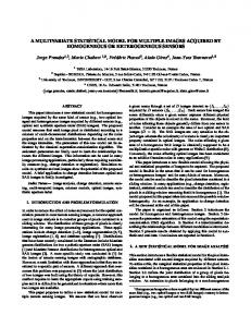
We compared the model results to an independent UHI intensity data set which was measured during the non-heating half year in 2002. The study area and the sampling method were the same as in the earlier cases, except that we used two cars to take temperature measurements at the same time in the two sectors, altogether 18 times (Fig. 2a). Then we calculated the spatial distribution of the difference between the measured (independent) UHI intensities and the predicted ones by our model (Fig. 2b). There is also a similarity between them but we can find three important areas where the ∆T anomaly is between 0.4ºC and 0.6ºC. In the northeastern and southern parts of the city the predicted values are lower than the measured ones (negative anomaly). At the western border of the investigated area the predicted values are higher than the measured ones (positive anomaly). However, these areas occupy only a minor part of the study area (about 5.5 cells, 6% of the total area). The areas characterized by the differences lower than 0.2ºC are significantly larger, covering altogether 55 cells (about 57%). (a)
(b) 0. 0
4. CONCLUSION 0.0
0.0
The following conclusions are reached from the analysis presented: (i) On the basis of our statistical analysis there is a strong linear relationship between the mean UHI intensity and the studied 0.0 urban parameters in both 0 0. season. 0 . 0 (ii) The model have described the spatial Fig. 2. (a) Spatial distribution of the measured mean max. UHI intensity (ºC) distribution of the real UHI during the non-heating season in 2002 and (b) spatial distribution of the intensity field in the study area rather correctly, difference of measured and predicted mean max. UHI intensity (ºC) during the because the areas same season in Szeged characterized by the differences lower than 0.2ºC cover the larger parts of the city (57 %). Nevertheless, there are some – but not significant – differences between the predicted and measured UHI fields which are caused by some possible errors in the temperature samplings, the low number of studied parameters and the considerable irregularities of the surface geometry. (iii) This model-building procedure, used to predict the UHI intensity, may be applicable for other cities of different size and even non-concentric shape, but for the true validation it is necessary to have complete databases of measured intensities for those cities. Acknowledgements: This research was supported by the grant of the Hungarian Scientific Research Fund (OTKA T/034161). The figures were drawn by Z. Sumeghy. References Barsi, A., 2000, ERDAS IMAGINE OrthoBase Modul (in Hungarian). Manuscript, Budapest. Bärring, L. and Mattsson, J. O., 1985, Canyon geometry, street temperatures and urban heat island in Malmö, Sweden. Int. J. Climatol., 5, 433-444. Eliasson, I., 1996, Urban nocturnal temperatures, street geometry and land use. Atmos. Environ., 30, 379-392. Gallo, K.P. and Owen, T.W., 1999, Satellite-based adjusments for the urban heat island temperature bias. J. Appl. Meteorol., 38, 806-813. Golany, G.S., 1996, Urban design morphology and thermal performance. Atmos. Environ., 30, 455-465. Grimmond, C. S. B., Zutter, H., Potter, S., Schoof, J. and Souch, C., 1999, Evaluation and application of automated methods for measuring sky view factors in urban areas. CD Proceed. ICB-ICUC, Sydney. Kuttler, W., Barlag, A-B and, Roßmann, F., 1996, Study of the thermal structure of a town in a narrow valley. Atmos. Environ., 30, 365-378. Miller, A. J., 2002, Subset Selection in Regression. Chapman&Hall/CRC, Boca Raton. Morris, C.J.G., Simmonds, I. and Plummer, N., 2001, Quantification of the influences of wind and cloud on the nocturnal urban heat island of a large city. J. Appl. Meteorol., 40, 169-182. Oke, T.R., 1981, Canyon geometry and the nocturnal urban heat island: comparison of scale model and field observations. J. Climatol., 1, 237-254. Oke, T.R., 1988, Street design and urban canopy layer climate. Energy and Buildings, 11, 103-113. Unger, J., Sumeghy, Z., Gulyas, A., Bottyan, Z. and Mucsi, L., 2001, Land-use and meteorological aspects of the urban heat island. Meteorol. Applications, 8, 189-194. Yamashita, S., Sekine, K., Shoda, M., Yamashita, K. and Hara, Y., 1986, On the relationships between heat island and sky view factor in the cities of Tama River Basin, Japan. Atmos. Environ., 20, 681-686.